Singular perturbation

Methods of analysis

A perturbed problem whose solution can be approximated on the whole problem domain, whether space or time, by a single asymptotic expansion has a regular perturbation. Most often in applications, an acceptable approximation to a regularly perturbed problem is found by simply replacing the small parameter ε by zero everywhere in the problem statement. This corresponds to taking only the first term of the expansion, yielding an approximation that converges, perhaps slowly, to the true solution as ε decreases. The solution to a singularly perturbed problem cannot be approximated in this way: As seen in the examples below, a singular perturbation generally occurs when a problem's small parameter multiplies its highest operator. Thus naively taking the parameter to be zero changes the very nature of the problem. In the case of differential equations, boundary conditions cannot be satisfied; in algebraic equations, the possible number of solutions is decreased.

Singular perturbation theory is a rich and ongoing area of exploration for mathematicians, physicists, and other researchers. The methods used to tackle problems in this field are many. The more basic of these include the method of matched asymptotic expansions and WKB approximation for spatial problems, and in time, the Poincaré-Lindstedt method, the method of multiple scales and periodic averaging.

For books on singular perturbation in ODE and PDE's, see for example Holmes, Introduction to Perturbation Methods, Hinch, Perturbation methods or Bender and Orszag, Advanced Mathematical Methods for Scientists and Engineers.

Examples of singular perturbative problems

Each of the examples described below shows how a naive perturbation analysis, which assumes that the problem is regular instead of singular, will fail. Some show how the problem may be solved by more sophisticated singular methods.

Vanishing coefficients in ordinary differential equations

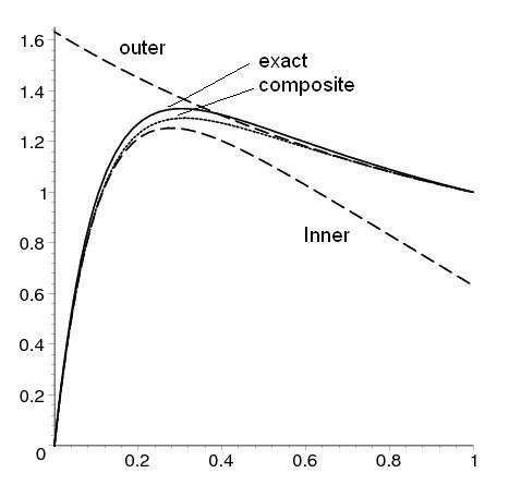
Differential equations that contain a small parameter that premultiplies the highest order term typically exhibit boundary layers, so that the solution evolves in two different scales. For example, consider the boundary value problem

Its solution when ε = 0.1 is the solid curve shown below. Note that the solution changes rapidly near the origin. If we naively set ε = 0 , we would get the solution labelled "outer" below which does not model the boundary layer, for which x is close to zero. For more details that show how to obtain the uniformly valid approximation, see method of matched asymptotic expansions.

Examples in time

An electrically driven robot manipulator can have slower mechanical dynamics and faster electrical dynamics, thus exhibiting two time scales. In such cases, we can divide the system into two subsystems, one corresponding to faster dynamics and other corresponding to slower dynamics, and then design controllers for each one of them separately. Through a singular perturbation technique, we can make these two subsystems independent of each other, thereby simplifying the control problem.

Consider a class of system described by following set of equations:

with 0 < ε < < 1 . The second equation indicates that the dynamics of x 2 is much faster than that of x 1 . A theorem due to Tikhonov states that, with the correct conditions on the system, it will initially and very quickly approximate the solution to the equations

on some interval of time and that, as ε decreases toward zero, the system will approach the solution more closely in that same interval.

Examples in space

In fluid mechanics, the properties of a slightly viscous fluid are dramatically different outside and inside a narrow boundary layer. Thus the fluid exhibits multiple spatial scales.

Reaction-diffusion systems in which one reagent diffuses much more slowly than another can form spatial patterns marked by areas where a reagent exists, and areas where it does not, with sharp transitions between them. In ecology, predator-prey models such as

where u is the prey and v is the predator, have been shown to exhibit such patterns.

Algebraic equations

Consider the problem of finding all roots of the polynomial p ( x ) = ε x 3 − x 2 + 1 . In the limit ε → 0 , this cubic degenerates into the quadratic 1 − x 2 with roots at x = ± 1 . Substituting a regular perturbation series:

x ( ε ) = x 0 + ε x 1 + ε 2 x 2 + ⋯

in the equation and equating equal powers of ε only yields corrections to these two roots:

x ( ε ) = ± 1 + 1 2 ε ± 5 8 ε 2 + ⋯

To find the other root, singular perturbation analysis must be used. We must then deal with the fact that the equation degenerates into a quadratic when we let ε tend to zero, in that limit one of the roots escapes to infinity. To prevent this root from becoming invisible to the perturbative analysis, we must rescale x to keep track with this escaping root so that in terms of the rescaled variables, it doesn't escape. We define a rescaled variable x = y ε ν where the exponent ν will be chosen such that we rescale just fast enough so that the root is at a finite value of y in the limit of ε to zero, but such that it doesn't collapse to zero where the other two roots will end up. In terms of y we have:

y 3 − ε ν − 1 y 2 + ε 3 ν − 1 = 0

We can see that for ν < 1 the y 3 is dominated by the lower degree terms, while at ν = 1 it becomes as dominant as the y 2 term while they both dominate the remaining term. This point where the highest order term will no longer vanish in the limit ε to zero by becoming equally dominant to another term, is called significant degeneration; this yields the correct rescaling to make the remaining root visible. This choice yields:

y 3 − y 2 + ε 2 = 0

Substituting the perturbation series:

y ( ε ) = y 0 + ε 2 y 1 + ε 4 y 2 + ⋯

yields:

y 0 3 − y 0 2 = 0

We're then interested in the root at y 0 = 1 ; the double root at y 0 = 0 are the two roots that we've found above that collapse to zero in the limit of an infinite rescaling. Calculating the first few terms of the series then yields:

x ( ε ) = y ( ε ) ε = 1 ε − ε − 2 ε 3 + ⋯