In numerical analysis, the Shanks transformation is a non-linear series acceleration method to increase the rate of convergence of a sequence. This method is named after Daniel Shanks, who rediscovered this sequence transformation in 1955. It was first derived and published by R. Schmidt in 1941.
For a sequence { a m } m ∈ N the series
A = ∑ m = 0 ∞ a m is to be determined. First, the partial sum A n is defined as:
A n = ∑ m = 0 n a m and forms a new sequence { A n } n ∈ N . Provided the series converges, A n will also approach the limit A as n → ∞ . The Shanks transformation S ( A n ) of the sequence A n is the new sequence defined by
S ( A n ) = A n + 1 A n − 1 − A n 2 A n + 1 − 2 A n + A n − 1 = A n + 1 − ( A n + 1 − A n ) 2 ( A n + 1 − A n ) − ( A n − A n − 1 ) where this sequence S ( A n ) often converges more rapidly than the sequence A n . Further speed-up may be obtained by repeated use of the Shanks transformation, by computing S 2 ( A n ) = S ( S ( A n ) ) , S 3 ( A n ) = S ( S ( S ( A n ) ) ) , etc.
Note that the non-linear transformation as used in the Shanks transformation is essentially the same as used in Aitken's delta-squared process so that as with Aitken's method, the right-most expression in S ( A n ) 's definition (i.e. S ( A n ) = A n + 1 − ( A n + 1 − A n ) 2 ( A n + 1 − A n ) − ( A n − A n − 1 ) ) is more numerically stable than the expression to its left (i.e. S ( A n ) = A n + 1 A n − 1 − A n 2 A n + 1 − 2 A n + A n − 1 ). Both Aitken's method and Shanks transformation operate on a sequence, but the sequence the Shanks transformation operates on is usually thought of as being a sequence of partial sums, although any sequence may be viewed as a sequence of partial sums.
As an example, consider the slowly convergent series
4 ∑ k = 0 ∞ ( − 1 ) k 1 2 k + 1 = 4 ( 1 − 1 3 + 1 5 − 1 7 + ⋯ ) which has the exact sum π ≈ 3.14159265. The partial sum A 6 has only one digit accuracy, while six-figure accuracy requires summing about 400,000 terms.
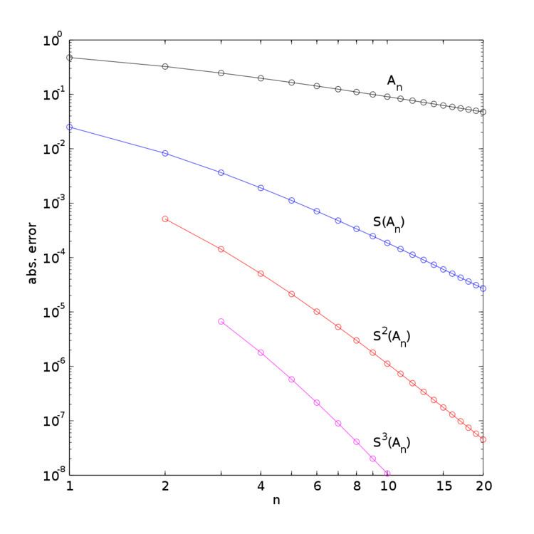
In the table below, the partial sums A n , the Shanks transformation S ( A n ) on them, as well as the repeated Shanks transformations S 2 ( A n ) and S 3 ( A n ) are given for n up to 12. The figure to the right shows the absolute error for the partial sums and Shanks transformation results, clearly showing the improved accuracy and convergence rate.
The Shanks transformation S ( A 1 ) already has two-digit accuracy, while the original partial sums only establish the same accuracy at A 24 . Remarkably, S 3 ( A 3 ) has six digits accuracy, obtained from repeated Shank transformations applied to the first seven terms A 0 , … , A 6 . As said before, A n only obtains 6-digit accuracy after about summing 400,000 terms.
The Shanks transformation is motivated by the observation that — for larger n — the partial sum A n quite often behaves approximately as
A n = A + α q n , with | q | < 1 so that the sequence converges transiently to the series result A for n → ∞ . So for n − 1 , n and n + 1 the respective partial sums are:
A n − 1 = A + α q n − 1 , A n = A + α q n and A n + 1 = A + α q n + 1 . These three equations contain three unknowns: A , α and q . Solving for A gives
A = A n + 1 A n − 1 − A n 2 A n + 1 − 2 A n + A n − 1 . In the (exceptional) case that the denominator is equal to zero: then A n = A for all n .
The generalized kth-order Shanks transformation is given as the ratio of the determinants:
S k ( A n ) = | A n − k ⋯ A n − 1 A n Δ A n − k ⋯ Δ A n − 1 Δ A n Δ A n − k + 1 ⋯ Δ A n Δ A n + 1 ⋮ ⋮ ⋮ Δ A n − 1 ⋯ Δ A n + k − 2 Δ A n + k − 1 | | 1 ⋯ 1 1 Δ A n − k ⋯ Δ A n − 1 Δ A n Δ A n − k + 1 ⋯ Δ A n Δ A n + 1 ⋮ ⋮ ⋮ Δ A n − 1 ⋯ Δ A n + k − 2 Δ A n + k − 1 | , with Δ A p = A p + 1 − A p . It is the solution of a model for the convergence behaviour of the partial sums A n with k distinct transients:
A n = A + ∑ p = 1 k α p q p n . This model for the convergence behaviour contains 2 k + 1 unknowns. By evaluating the above equation at the elements A n − k , A n − k + 1 , … , A n + k and solving for A , the above expression for the kth-order Shanks transformation is obtained. The first-order generalized Shanks transformation is equal to the ordinary Shanks transformation: S 1 ( A n ) = S ( A n ) .
The generalized Shanks transformation is closely related to Padé approximants and Padé tables.