
 | ||
In statistics, Smooth Transition Autoregressive (STAR) models are typically applied to time series data as an extension of autoregressive models, in order to allow for higher degree of flexibility in model parameters through a smooth transition.
Contents
- AutoRegressive Models
- STAR as an Extension of the AutoRegressive Model
- Basic Structure
- Transition Function
- References
Given a time series of data xt, the STAR model is a tool for understanding and, perhaps, predicting future values in this series, assuming that the behaviour of the series changes depending on the value of the transition variable. The transition might depend on the past values of the x series (similar to the SETAR models), or exogenous variables.
The model consists of 2 autoregressive (AR) parts linked by the transition function. The model is usually referred to as the STAR(p) models proceeded by the letter describing the transition function (see below) and p is the order of the autoregressive part. Most popular transition function include exponential function and first and second-order logistic functions. They give rise to Logistic STAR (LSTAR) and Exponential STAR (ESTAR) models.
AutoRegressive Models
Consider a simple AR(p) model for a time series yt
where:
written in a following vector form:
where:
STAR as an Extension of the AutoRegressive Model
STAR models were introduced and comprehensively developed by Kung-sik Chan and Howell Tong in 1986 (esp. p. 187), in which the same acronym was used. It originally stands for Smooth Threshold AutoRegressive. For some background history, see Tong (2011, 2012). The models can be thought of in terms of extension of autoregressive models discussed above, allowing for changes in the model parameters according to the value of weakly exogenous transition variable zt.
Defined in this way, STAR model can be presented as follows:
where:
Basic Structure
They can be understood as two-regime SETAR model with smooth transition between regimes, or as continuum of regimes. In both cases the presence of the transition function is the defining feature of the model as it allows for changes in values of the parameters.
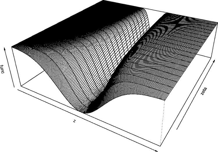
Transition Function
Three basic transition functions and the name of resulting models are: