
 | ||
In statistics, Redescending M-estimators are Ψ-type M-estimators which have ψ functions that are non-decreasing near the origin, but decreasing toward 0 far from the origin. Their ψ functions can be chosen to redescend smoothly to zero, so that they usually satisfy ψ(x) = 0 for all x with |x| > r, where r is referred to as the minimum rejection point.
Contents
Due to these properties of the ψ function, these kinds of estimators are very efficient, have a high breakdown point and, unlike other outlier rejection techniques, they do not suffer from a masking effect. They are efficient because they completely reject gross outliers, and do not completely ignore moderately large outliers (like median).
Advantages
Redescending M-estimators have high breakdown points (close to 0.5), and their Ψ function can be chosen to redescend smoothly to 0. This means that moderately large outliers are not ignored completely, and greatly improves the efficiency of the redescending M-estimator.
The redescending M-estimators are slightly more efficient than the Huber estimator for several symmetric, wider tailed distributions, but about 20% more efficient than the Huber estimator for the Cauchy distribution. This is because they completely reject gross outliers, while the Huber estimator effectively treats these the same as moderate outliers.
As other M-estimators, but unlike other outlier rejection techniques, they do not suffer from masking effects.
Disadvantages
The M-estimating equation for a redescending estimator may not have a unique solution.
Choosing redescending Ψ functions
When choosing a redescending Ψ function, care must be taken such that it does not descend too steeply, which may have a very bad influence on the denominator in the expression for the asymptotic variance
where F is the mixture model distribution.
This effect is particularly harmful when a large negative value of ψ'(x) combines with a large positive value of ψ2(x), and there is a cluster of outliers near x.
Examples
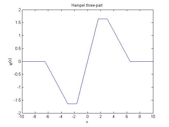
1. Hampel's three-part M estimators have Ψ functions which are odd functions and defined for any x by:
This function is plotted in the following figure for a=1.645, b=3 and r=6.5.
2. Tukey's biweight or bisquare M estimators have Ψ functions for any positive k, which defined by:
This function is plotted in the following figure for k=5.
3. Andrew's sine wave M estimator has the following Ψ function:
This function is plotted in the following figure.