Random sample consensus

Example

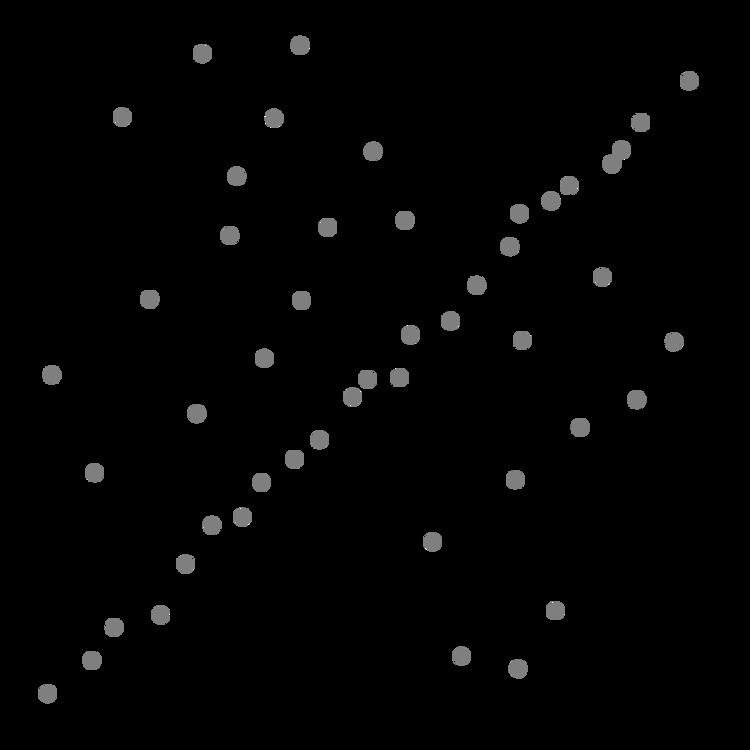
A simple example is fitting of a line in two dimensions to a set of observations. Assuming that this set contains both inliers, i.e., points which approximately can be fitted to a line, and outliers, points which cannot be fitted to this line, a simple least squares method for line fitting will generally produce a line with a bad fit to the inliers. The reason is that it is optimally fitted to all points, including the outliers. RANSAC, on the other hand, can produce a model which is only computed from the inliers, provided that the probability of choosing only inliers in the selection of data is sufficiently high. There is no guarantee for this situation, however, and there are a number of algorithm parameters which must be carefully chosen to keep the level of probability reasonably high.

Overview

The RANSAC algorithm is a learning technique to estimate parameters of a model by random sampling of observed data. Given a dataset whose data elements contain both inliers and outliers, RANSAC uses the voting scheme to find the optimal fitting result. Data elements in the dataset are used to vote for one or multiple models. The implementation of this voting scheme is based on two assumptions: that the noisy features will not vote consistently for any single model (few outliers) and there are enough features to agree on a good model (few missing data). The RANSAC algorithm is essentially composed of two steps that are iteratively repeated:

1. In the first step, a sample subset containing minimal data items is randomly selected from the input dataset. A fitting model and the corresponding model parameters are computed using only the elements of this sample subset. The cardinality of the sample subset is the smallest sufficient to determine the model parameters.
2. In the second step, the algorithm checks which elements of the entire dataset are consistent with the model instantiated by the estimated model parameters obtained from the first step. A data element will be considered as an outlier if it does not fit the fitting model instantiated by the set of estimated model parameters within some error threshold that defines the maximum deviation attributable to the effect of noise.

The set of inliers obtained for the fitting model is called consensus set. The RANSAC algorithm will iteratively repeat the above two steps until the obtained consensus set in certain iteration has enough inliers.

The input to the RANSAC algorithm is a set of observed data values, a way of fitting some kind of model to the observations, and some confidence parameters. RANSAC achieves its goal by repeating the following steps:

1. Select a random subset of the original data. Call this subset the hypothetical inliers.
2. A model is fitted to the set of hypothetical inliers.
3. All other data are then tested against the fitted model. Those points that fit the estimated model well, according to some model-specific loss function, are considered as part of the consensus set.
4. The estimated model is reasonably good if sufficiently many points have been classified as part of the consensus set.
5. Afterwards, the model may be improved by reestimating it using all members of the consensus set.

This procedure is repeated a fixed number of times, each time producing either a model which is rejected because too few points are part of the consensus set, or a refined model together with a corresponding consensus set size. In the latter case, we keep the refined model if its consensus set is larger than the previously saved model.

Algorithm

The generic RANSAC algorithm works as follows:

Given: data – a set of observed data points model – a model that can be fitted to data points n – the minimum number of data values required to fit the model k – the maximum number of iterations allowed in the algorithm t – a threshold value for determining when a data point fits a model d – the number of close data values required to assert that a model fits well to data Return: bestfit – model parameters which best fit the data (or nul if no good model is found) iterations = 0 bestfit = nul besterr = something really large while iterations < k { maybeinliers = n randomly selected values from data maybemodel = model parameters fitted to maybeinliers alsoinliers = empty set for every point in data not in maybeinliers { if point fits maybemodel with an error smaller than t add point to alsoinliers } if the number of elements in alsoinliers is > d { % this implies that we may have found a good model % now test how good it is bettermodel = model parameters fitted to all points in maybeinliers and alsoinliers thiserr = a measure of how well model fits these points if thiserr < besterr { bestfit = bettermodel besterr = thiserr } } increment iterations } return bestfit

Matlab implementation

A Matlab implementation of 2D line fitting using the RANSAC algorithm:

Parameters

The values of parameters t and d have to be determined from specific requirements related to the application and the data set, possibly based on experimental evaluation. The parameter k (the number of iterations), however, can be determined from a theoretical result. Let p be the probability that the RANSAC algorithm in some iteration selects only inliers from the input data set when it chooses the n points from which the model parameters are estimated. When this happens, the resulting model is likely to be useful so p gives the probability that the algorithm produces a useful result. Let w be the probability of choosing an inlier each time a single point is selected, that is,

w = number of inliers in data / number of points in data

A common case is that w is not well known beforehand, but some rough value can be given. Assuming that the n points needed for estimating a model are selected independently, w n is the probability that all n points are inliers and 1 − w n is the probability that at least one of the n points is an outlier, a case which implies that a bad model will be estimated from this point set. That probability to the power of k is the probability that the algorithm never selects a set of n points which all are inliers and this must be the same as 1 − p . Consequently,

1 − p = ( 1 − w n ) k

which, after taking the logarithm of both sides, leads to

k = log ⁡ ( 1 − p ) log ⁡ ( 1 − w n )

This result assumes that the n data points are selected independently, that is, a point which has been selected once is replaced and can be selected again in the same iteration. This is often not a reasonable approach and the derived value for k should be taken as an upper limit in the case that the points are selected without replacement. For example, in the case of finding a line which fits the data set illustrated in the above figure, the RANSAC algorithm typically chooses two points in each iteration and computes maybe_model as the line between the points and it is then critical that the two points are distinct.

To gain additional confidence, the standard deviation or multiples thereof can be added to k. The standard deviation of k is defined as

SD ⁡ ( k ) = 1 − w n w n

Advantages and disadvantages

An advantage of RANSAC is its ability to do robust estimation of the model parameters, i.e., it can estimate the parameters with a high degree of accuracy even when a significant number of outliers are present in the data set. A disadvantage of RANSAC is that there is no upper bound on the time it takes to compute these parameters (except exhaustion). When the number of iterations computed is limited the solution obtained may not be optimal, and it may not even be one that fits the data in a good way. In this way RANSAC offers a trade-off; by computing a greater number of iterations the probability of a reasonable model being produced is increased. Moreover, RANSAC is not always able to find the optimal set even for moderately contaminated sets and it usually performs badly when the number of inliers is less than 50%. Optimal RANSAC was proposed to handle both these problems and is capable of finding the optimal set for heavily contaminated sets, even for an inlier ratio under 5%. Another disadvantage of RANSAC is that it requires the setting of problem-specific thresholds.

RANSAC can only estimate one model for a particular data set. As for any one-model approach when two (or more) model instances exist, RANSAC may fail to find either one. The Hough transform is one alternative robust estimation technique that may be useful when more than one model instance is present. Another approach for multi model fitting is known as PEARL, which combines model sampling from data points as in RANSAC with iterative re-estimation of inliers and the multi-model fitting being formulated as an optimization problem with a global energy functional describing the quality of the overall solution.

Applications

The RANSAC algorithm is often used in computer vision, e.g., to simultaneously solve the correspondence problem and estimate the fundamental matrix related to a pair of stereo cameras.

Development and improvements

Since 1981 RANSAC has become a fundamental tool in the computer vision and image processing community. In 2006, for the 25th anniversary of the algorithm, a workshop was organized at the International Conference on Computer Vision and Pattern Recognition (CVPR) to summarize the most recent contributions and variations to the original algorithm, mostly meant to improve the speed of the algorithm, the robustness and accuracy of the estimated solution and to decrease the dependency from user defined constants.

As pointed out by Torr et al. , RANSAC can be sensitive to the choice of the correct noise threshold that defines which data points fit a model instantiated with a certain set of parameters. If such threshold is too large, then all the hypotheses tend to be ranked equally (good). On the other hand, when the noise threshold is too small, the estimated parameters tend to be unstable ( i.e. by simply adding or removing a datum to the set of inliers, the estimate of the parameters may fluctuate). To partially compensate for this undesirable effect, Torr et al. proposed two modification of RANSAC called MSAC (M-estimator SAmple and Consensus) and MLESAC (Maximum Likelihood Estimation SAmple and Consensus). The main idea is to evaluate the quality of the consensus set ( i.e. the data that fit a model and a certain set of parameters) calculating its likelihood (whereas in the original formulation by Fischler and Bolles the rank was the cardinality of such set). An extension to MLESAC which takes into account the prior probabilities associated to the input dataset is proposed by Tordoff. The resulting algorithm is dubbed Guided-MLESAC. Along similar lines, Chum proposed to guide the sampling procedure if some a priori information regarding the input data is known, i.e. whether a datum is likely to be an inlier or an outlier. The proposed approach is called PROSAC, PROgressive SAmple Consensus.

Chum et al. also proposed a randomized version of RANSAC called R-RANSAC to reduce the computational burden to identify a good CS. The basic idea is to initially evaluate the goodness of the currently instantiated model using only a reduced set of points instead of the entire dataset. A sound strategy will tell with high confidence when it is the case to evaluate the fitting of the entire dataset or when the model can be readily discarded. It is reasonable to think that the impact of this approach is more relevant in cases where the percentage of inliers is large. The type of strategy proposed by Chum et al. is called preemption scheme. Nistér proposed a paradigm called Preemptive RANSAC that allows real time robust estimation of the structure of a scene and of the motion of the camera. The core idea of the approach consists in generating a fixed number of hypothesis so that the comparison happens with respect to the quality of the generated hypothesis rather than against some absolute quality metric.

Other researchers tried to cope with difficult situations where the noise scale is not known and/or multiple model instances are present. The first problem has been tackled in the work by Wang and Suter. Toldo et al. represent each datum with the characteristic function of the set of random models that fit the point. Then multiple models are revealed as clusters which group the points supporting the same model. The clustering algorithm, called J-linkage, does not require prior specification of the number of models, nor does it necessitate manual parameters tuning.

RANSAC has also been tailored for recursive state estimation applications, where the input measurements are corrupted by outliers and Kalman filter approaches, which rely on a Gaussian distribution of the measurement error, are doomed to fail. Such an approach is dubbed KALMANSAC.

Related methods

MLESAC (Maximum Likelihood Estimate SAmple Consensus) – maximizes the likelihood that the data was generated from the sample-fitted model, e.g. a mixture model of inliers and outliers

MAPSAC (Maximum A Posterior SAmple Consensus) – extends MLESAC to incorporate a prior probability of the parameters to be fitted and maximizes the posterior probability

KALMANSAC – causal inference of the state of a dynamical system