
 | ||
Sonja barkhofen quantum walks in time
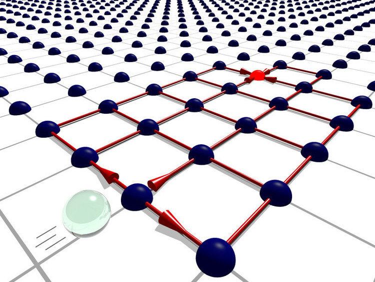
In quantum computing, quantum walks are the quantum analogue of classical random walks. Analogous to the classical random walk, where the walker's current state is described by a probability distribution over positions, the walker in a quantum walk is in a superposition of positions.
Contents
- Sonja barkhofen quantum walks in time
- Dr hab magdalena stobi ska quantum walks mastering the complexity and the uncomputable
- Motivation
- Relation to classical random walks
- Continuous time
- Discrete time
- References
Like classical random walks, there are two types of quantum walks: discrete-time quantum walks and continuous-time quantum walks.
Dr hab magdalena stobi ska quantum walks mastering the complexity and the uncomputable
Motivation
Quantum walks are motivated by the widespread use of classical random walks in the design of randomized algorithms, and are part of several quantum algorithms. For some oracular problems, quantum walks provide an exponential speedup over any classical algorithm. Quantum walks also give polynomial speedups over classical algorithms for many practical problems, such as the element distinctness problem, the triangle finding problem, and evaluating NAND trees. The well-known Grover search algorithm can also be viewed as a quantum walk algorithm.
Relation to classical random walks
Quantum walks exhibit very different features from classical random walks. In particular, they do not converge to limiting distributions and due to the power of quantum interference they may spread significantly faster or slower than their classical equivalents.
Continuous time
Under particular conditions, continuous-time quantum walks can provide a model for universal quantum computation. This does not necessarily imply uniformality.
Discrete time
A quantum walk in discrete time is specified by a coin and shift operator, which are applied repeatedly. The following example is instructive here. Imagine a particle on a line (one-dimensional model) with an inner spin-1/2-degree of freedom, i.e. its state can be described by a product state of a spin state
Consider what happens when we discretize a massive Dirac operator over one spatial dimension. In the absence of a mass term, we have left-movers and right-movers. They can be characterized by an internal degree of freedom, "spin" or a "coin". When we turn on a mass term, this corresponds to a rotation in this internal "coin" space. A quantum walk corresponds to iterating the shift and coin operators repeatedly.
This is very much like Richard Feynman's model of an electron in 1 (one) spatial and 1 (one) time dimension. He summed up the zigzagging paths, with left-moving segments corresponding to one spin (or coin), and right-moving segments to the other. See Feynman checkerboard for more details.
The transition probability for a 1-dimensional quantum walk behaves like the Hermite functions which (1) asymptotically oscillate in the classically allowed region, (2) is approximated by the Airy function around the wall of the potential, and (3) exponentially decay in the classically hidden region.