Neha Patil (Editor)

Quantum pendulum

Updated on
Edit
Like
Comment
Share on FacebookTweet on TwitterShare on LinkedInShare on Reddit
Quantum pendulum

The quantum pendulum is fundamental in understanding hindered internal rotations in chemistry, quantum features of scattering atoms, as well as numerous other quantum phenomena. Though a pendulum not subject to the small-angle approximation has an inherent nonlinearity, the Schrödinger equation for the quantized system can be solved relatively easily.

Contents

Schrödinger equation

Using Lagrangian theory from classical mechanics, one can develop a Hamiltonian for the system. A simple pendulum has one generalized coordinate (the angular displacement ϕ ) and two constraints (the length of the string and the plane of motion). The kinetic and potential energies of the system can be found to be

T = 1 2 m l 2 ϕ ˙ 2 , U = m g l ( 1 cos ϕ ) .

This results in the Hamiltonian

H ^ = p ^ 2 2 m l 2 + m g l ( 1 cos ϕ ) .

The time-dependent Schrödinger equation for the system is

i d Ψ d t = 2 2 m l 2 d 2 Ψ d ϕ 2 + m g l ( 1 cos ϕ ) Ψ .

One must solve the time-independent Schrödinger equation to find the energy levels and corresponding eigenstates. This is best accomplished by changing the independent variable as follows:

η = ϕ + π , Ψ = ψ e i E t / , E ψ = 2 2 m l 2 d 2 ψ d η 2 + m g l ( 1 + cos η ) ψ .

This is simply Mathieu's equation

d 2 ψ d η 2 + ( 2 m E l 2 2 2 m 2 g l 3 2 2 m 2 g l 3 2 cos η ) ψ = 0 ,

where the solutions are Mathieu functions.

Energies

Given q , for countably many special values of a , called characteristic values, the Mathieu equation admits solutions that are periodic with period 2 π . The characteristic values of the Mathieu cosine, sine functions respectively are written a n ( q ) , b n ( q ) , where n is a natural number. The periodic special cases of the Mathieu cosine and sine functions are often written C E ( n , q , x ) , S E ( n , q , x ) respectively, although they are traditionally given a different normalization (namely, that their L2 norm equal π ).

The boundary conditions in the quantum pendulum imply that a n ( q ) , b n ( q ) are as follows for a given q:

d 2 ψ d η 2 + ( 2 m E l 2 2 2 m 2 g l 3 2 2 m 2 g l 3 2 cos η ) ψ = 0 , a n ( q ) , b n ( q ) = 2 m E l 2 2 2 m 2 g l 3 2 .

The energies of the system, E = m g l + 2 a n ( q ) , b n ( q ) 2 m l 2 for even/odd solutions respectively, are quantized based on the characteristic values found by solving the Mathieu equation.

The effective potential depth can be defined as

q = m 2 g l 3 2 .

A deep potential yields the dynamics of a particle in an independent potential. In contrast, in a shallow potential, Bloch waves, as well as quantum tunneling, become of importance.

General solution

The general solution of the above differential equation for a given value of a and q is a set of linearly independent Mathieu cosines and Mathieu sines, which are even and odd solutions respectively. In general, the Mathieu functions are aperiodic; however, for characteristic values of a n ( q ) , b n ( q ) , the Mathieu cosine and sine become periodic with a period of 2 π .

Eigenstates

For positive values of q, the following is true:

C ( a n ( q ) , q , x ) = C E ( n , q , x ) C E ( n , q , 0 ) , S ( b n ( q ) , q , x ) = S E ( n , q , x ) S E ( n , q , 0 ) .

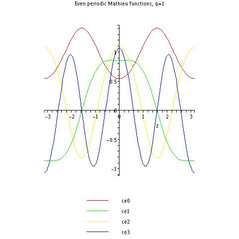
Here are the first few periodic Mathieu cosine functions for q = 1:

Note that, for example, C E ( 1 , 1 , x ) (green) resembles a cosine function, but with flatter hills and shallower valleys.

References

Quantum pendulum Wikipedia