The exact thin plate energy functional (TPEF) for a function f ( x , y ) is
∫ y 0 y 1 ∫ x 0 x 1 ( κ 1 2 + κ 2 2 ) g d x d y where κ 1 and κ 2 are the principal curvatures of the surface mapping f at the point ( x , y ) . This is the surface integral of κ 1 2 + κ 2 2 , hence the g in the integrand.
Minimizing the exact thin plate energy functional would result in a system of non-linear equations. So in practice, an approximation that results in linear systems of equations is often used. The approximation is derived by assuming that the gradient of f is 0. At any point where f x = f y = 0 , the first fundamental form g i j of the surface mapping f is the identity matrix and the second fundamental form b i j is
( f x x f x y f x y f y y ) .
We can use the formula for mean curvature H = b i j g i j / 2 to determine that H = ( f x x + f y y ) / 2 and the formula for Gaussian curvature K = b / g (where b and g are the determinants of the second and first fundamental forms, respectively) to determine that K = f x x f y y − ( f x y ) 2 . Since H = ( k 1 + k 2 ) / 2 and K = k 1 k 2 , the integrand of the exact TPEF equals 4 H 2 − 2 K . The expressions we just computed for the mean curvature and Gaussian curvature as functions of partial derivatives of f show that the integrand of the exact TPEF is
4 H 2 − 2 K = ( f x x + f y y ) 2 − 2 ( f x x f y y − f x y 2 ) = f x x 2 + 2 f x y 2 + f y y 2 . So the approximate thin plate energy functional is
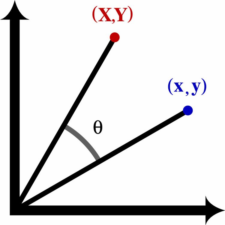
J [ f ] = ∫ y 0 y 1 ∫ x 0 x 1 f x x 2 + 2 f x y 2 + f y y 2 d x d y . The TPEF is rotationally invariant. This means that if all the points of the surface z ( x , y ) are rotated by an angle θ about the z -axis, the TPEF at each point ( x , y ) of the surface equals the TPEF of the rotated surface at the rotated ( x , y ) . The formula for a rotation by an angle θ about the z -axis is
The fact that the z value of the surface at ( x , y ) equals the z value of the rotated surface at the rotated ( x , y ) is expressed mathematically by the equation
Z ( X , Y ) = z ( x , y ) = ( z ∘ x y ) ( X , Y ) where x y is the inverse rotation, that is, x y ( X , Y ) = R − 1 ( X , Y ) T = R T ( X , Y ) T . So Z = z ∘ x y and the chain rule implies
In equation (2), Z 0 means Z X , Z 1 means Z Y , z 0 means z x , and z 1 means z y . Equation (2) and all subsequent equations in this section use non-tensor summation convention, that is, sums are taken over repeated indices in a term even if both indices are subscripts. The chain rule is also needed to differentiate equation (2) since z j is actually the composition z j ∘ x y :
Z i k = z j l R k l R i j .
Swapping the index names j and k yields
Expanding the sum for each pair i , j yields
Z X X = R 00 2 z x x + 2 R 00 R 01 z x y + R 01 2 z y y , Z X Y = R 00 R 10 z x x + ( R 00 R 11 + R 01 R 10 ) z x y + R 01 R 11 z y y , Z Y Y = R 10 2 z x x + 2 R 10 R 11 z x y + R 11 2 z y y . Computing the TPEF for the rotated surface yields
Inserting the coefficients of the rotation matrix R from equation (1) into the right-hand side of equation (4) simplifies it to z x x 2 + 2 z x y 2 + z y y 2 .
The approximate thin plate energy functional can be used to fit B-spline surfaces to scattered 1D data on a 2D grid (for example, digital terrain model data). Call the grid points ( x i , y i ) for i = 1 … N (with x i ∈ [ a , b ] and y i ∈ [ c , d ] ) and the data values z i . In order to fit a uniform B-spline f ( x , y ) to the data, the equation
(where λ is the "smoothing parameter") is minimized. Larger values of λ result in a smoother surface and smaller values result in a more accurate fit to the data. The following images illustrate the results of fitting a B-spline surface to some terrain data using this method.
The thin plate smoothing spline also minimizes equation (5), but it is much more expensive to compute than a B-spline and not as smooth (it is only C 1 at the "centers" and has unbounded second derivatives there).