Percolation threshold

Percolation models

The most common percolation model is to take a regular lattice, like a square lattice, and make it into a random network by randomly "occupying" sites (vertices) or bonds (edges) with a statistically independent probability p. At a critical threshold p_c, large clusters and long-range connectivity first appears, and this is called the percolation threshold. Depending on the method for obtaining the random network, one distinguishes between the site percolation threshold and the bond percolation threshold. More general systems have several probabilities p₁, p₂, etc., and the transition is characterized by a critical surface or manifold. One can also consider continuum systems, such as overlapping disks and spheres placed randomly, or the negative space (Swiss-cheese models).

In the systems described so far, it has been assumed that the occupation of a site or bond is completely random—this is the so-called Bernoulli percolation. For a continuum system, random occupancy corresponds to the points being placed by a Poisson process. Further variations involve correlated percolation, such as percolation clusters related to Ising and Potts models of ferromagnets, in which the bonds are put down by the Fortuin-Kasteleyn method. In bootstrap or k-sat percolation, sites and/or bonds are first occupied and then successively culled from a system if a site does not have at least k neighbors. Another important model of percolation, in a different universality class altogether, is directed percolation, where connectivity along a bond depends upon the direction of the flow.

Over the last several decades, a tremendous amount of work has gone into finding exact and approximate values of the percolation thresholds for a variety of these systems. Exact thresholds are only known for certain two-dimensional lattices that can be broken up into a self-dual array, such that under a triangle-triangle transformation, the system remains the same. Studies using numerical methods have led to numerous improvements in algorithms and several theoretical discoveries.

The notation such as (4,8²) comes from Grünbaum and Shephard, and indicates that around a given vertex, going in the clockwise direction, one encounters first a square and then two octagons. Besides the eleven Archimedean lattices composed of regular polygons with every site equivalent, many other more complicated lattices with sites of different classes have been studied.

Error bars in the last digit or digits are shown by numbers in parentheses. Thus, 0.729724(3) signifies 0.729724 ± 0.000003, and 0.74042195(80) signifies 0.74042195 ± 0.00000080. The error bars variously represent one or two standard deviations in net error (including statistical and expected systematic error), or an empirical confidence interval.

Thresholds on Archimedean lattices

This is a picture of the 11 Archimedean Lattices or uniform tilings, in which all polygons are regular and each vertex is surrounded by the same sequence of polygons. The notation (3⁴, 6) for example means that every vertex is surrounded by four triangles and one hexagon. Drawings from . See also Uniform Tilings.

Note: sometimes "hexagonal" is used in place of honeycomb, although in some fields, a triangular lattice is also called a hexagonal lattice. z = bulk coordination number.

Square lattice with complex neighborhoods

2N = nearest neighbors, 3N = next-nearest neighbors, 4N = next-next-nearest neighbors, etc. These are called NN, 2NN, 3NN respectively in the 3D versions below.

For more neighbors, see

Archimedean Duals (Laves Lattices)

Laves lattices are the duals to the Archimedean lattices. Drawings from. See also Uniform Tilings.

Site bond percolation (both thresholds apply simultaneously to one system).

* For more values, see An Investigation of site-bond percolation

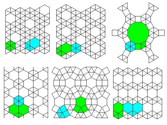
2-Uniform Lattices

Top 3 Lattices: #13 #12 #36
Bottom 3 Lattices: #34 #37 #11

Top 2 Lattices: #35 #30
Bottom 2 Lattices: #41 #42

Top 4 Lattices: #22 #23 #21 #20
Bottom 3 Lattices: #16 #17 #15

Top 2 Lattices: #31 #32
Bottom Lattice: #33

This figure shows the 2-uniform lattice #37 in the isoradial representation in which each polygon is inscribed in a circle of unit radius. The squares in the 2-uniform lattice must now be represented as rectangles in order to satisfy the isoradial condition. The lattice is shown by black edges, and the dual lattice by red dashed lines. The green circles show the isoradial constraint on both the original and dual lattices. The yellow polygons highlight the three types of polygons on the lattice, and the pink polygons highlight the two types of polygons on the dual lattice. The lattice has vertex types (1/2)(3³,4²) + (1/2)(3,4,6,4), while the dual lattice has vertex types (1/15)(4⁶)+(6/15)(4²,5²)+(2/15)(5³)+(6/15)(5²,4). The critical point is where the longer bonds (on both the lattice and dual lattice) have occupation probability p = 2 sin (π/18) = 0.347296... which is the bond percolation threshold on a triangular lattice, and the shorter bonds have occupation probability 1 - 2 sin(π/18) = 0.652703..., which is the bond percolation on a hexagonal lattice. These results follow from the isoradial condition but also follow from applying the star-triangle transformation to certain stars on the honeycomb lattice. Finally, it can be generalized to having three different probabilities in the three different directions, p₁, p₂ and p₃ for the long bonds, and 1 - p₁, 1 - p₂, and 1 - p₃ for the short bonds, where p₁, p₂ and p₃ satisfy the critical surface for the inhomogeneous triangular lattice.

Thresholds on 2D bow-tie and martini lattices

To the left, center, and right are: the martini lattice, the martini-A lattice, the martini-B lattice. Below: the martini covering/medial lattice, same as the 2x2, 1x1 subnet for kagome-type lattices (removed).

Some other examples of generalized bow-tie lattices (a-d) and the duals of the lattices (e-h)

Thresholds on 2D covering, medial, and matching lattices

(4, 6, 12) covering/medial lattice

(4, 8²) covering/medial lattice

(3,12²) covering/medial lattice (in light grey), equivalent to the kagome (2 x 2) subnet, and in black, the dual of these lattices.

(left) (3,4,6,4) covering/medial lattice, (right) (3,4,6,4) medial dual, shown in red, with medial lattice in light gray behind it

Thresholds on subnet lattices

The 2 x 2, 3 x 3, and 4 x 4 subnet kagome lattices. The 2 × 2 subnet is also known as the "triangular kagome" lattice

Thresholds of random sequentially adsorbed objects

The threshold gives the fraction of sites occupied by the objects when site percolation first takes place (not at full jamming). For longer dimers see Ref.

Thresholds of full dimer coverings of two dimensional lattices

Here, we are dealing with networks that are obtained by covering a lattice with dimers, and then consider bond percolation on the remaining bonds. In discrete mathematics, this problem is known as the 'perfect matching' or the 'dimer covering' problem.

Thresholds of polymers (random walks) on a square lattice

System is composed of ordinary (non-avoiding) random walks of length l on the square lattice.

Thresholds for 2D continuum models

η c = π r 2 N / L 2 equals critical total area for disks, where N is the number of objects and L is the system size.

η c = π a b N / L 2 for ellipses of semi-major and semi-minor axes of a and b, respectively. Aspect ratio ϵ = a / b with a > b .

η c = ℓ m N / L 2 for rectangles of dimensions ℓ and m . Aspect ratio ϵ = ℓ / m with ℓ > m .

η c = π x N / ( 4 L 2 ( x − 2 ) ) for power-law distributed disks with Prob(radius ≥ R ) = R − x , R ≥ 1 .

ϕ c = 1 − e − η c equals critical area fraction.

n c = ℓ 2 N / L 2 equals number of objects of maximum length ℓ = 2 a per unit area.

For ellipses, n c = ( 4 ϵ / π ) η c

For void percolation, ϕ c = e − η c is the critical void fraction.

For more ellipse values, see

For more rectangle values, see

Thresholds on 2D random and quasi-lattices

*Theoretical estimate

Thresholds on slabs

More for SC open b.c. in Ref.

h is the thickness of the slab, h x ∞ x ∞.

Thresholds on 3D lattices

Filling factor = fraction of space filled by touching spheres at every lattice site (for systems with uniform bond length only). Also called Atomic Packing Factor.

Filling fraction (or Critical Filling Fraction) = filling factor * p_c(site).

NN = nearest neighbor, 2NN = next-nearest neighbor, 3NN = next-next-nearest neighbor, etc.

Question: the bond thresholds for the HCP and FCC lattice agree within the small statistical error. Are they identical, and if not, how far apart are they? Which threshold is expected to be bigger? Similarly for the ice and diamond lattices. See

Thresholds for 3D continuum models

All overlapping except for jammed spheres and polymer matrix.

η c = ( 4 / 3 ) π r 3 N / L 3 is the total volume, where N is the number of objects and L is the system size.

ϕ c = 1 − e − η c is the critical volume fraction.

For disks and plates, these are effective volumes and volume fractions.

For void ("Swiss-Cheese" model), ϕ c = e − η c is the critical void fraction.

For more results on void percolation around ellipsoids and elliptical plates, see.

For more ellipsoid percolation values see

Thresholds for 3D correlated percolation

Continuum models in higher dimensions

η c = ( π d / 2 / Γ [ d / 2 + 1 ] ) r d N / L d .

In 4d, η c = ( 1 / 2 ) π 2 r 4 N / L 4 .

In 5d, η c = ( 8 / 15 ) π 2 r 5 N / L 5 .

In 6d, η c = ( 1 / 6 ) π 3 r 6 N / L 6 .

ϕ c = 1 − e − η c is the critical volume fraction.

For void models, ϕ c = e − η c is the critical void fraction, and η c is the total volume of the overlapping objects

Thresholds on hyperbolic, hierarchical, and tree lattices

Note: {m,n} is the Schläfli symbol, signifying a hyperbolic lattice in which n regular m-gons meet at every vertex

Cayley tree (Bethe lattice) with coordination number z: p_c= 1 / (z - 1)

Cayley tree with a distribution of z with mean z ¯ , mean-square z 2 ¯ : p_c= z ¯ / ( z 2 ¯ − z ¯ ) (site or bond threshold)

Thresholds for directed percolation

nn = nearest neighbors. For a (d+1)-dimensional hypercubic system, the hypercube is in d dimensions and the time direction points to the 2D nearest neighbors.

Exact critical manifolds of inhomogeneous systems

Inhomogeneous triangular lattice bond percolation

1 − p 1 − p 2 − p 3 + p 1 p 2 p 3 = 0

Inhomogeneous honeycomb lattice bond percolation = kagome lattice site percolation

1 − p 1 p 2 − p 1 p 3 − p 2 p 3 + p 1 p 2 p 3 = 0

Inhomogeneous (3,12^2) lattice, site percolation

1 − 3 ( s 1 s 2 ) 2 + ( s 1 s 2 ) 3 = 0 , or s 1 s 2 = 1 − 2 sin ⁡ ( π / 18 )

Inhomogeneous union-jack lattice, site percolation with probabilities p 1 , p 2 , p 3 , p 4

p 3 = 1 − p 1 ; p 4 = 1 − p 2

Inhomogeneous martini lattice, bond percolation 1 − ( p 1 p 2 r 3 + p 2 p 3 r 1 + p 1 p 3 r 2 ) − ( p 1 p 2 r 1 r 2 + p 1 p 3 r 1 r 3 + p 2 p 3 r 2 r 3 ) + p 1 p 2 p 3 ( r 1 r 2 + r 1 r 3 + r 2 r 3 ) + r 1 r 2 r 3 ( p 1 p 2 + p 1 p 3 + p 2 p 3 ) − 2 p 1 p 2 p 3 r 1 r 2 r 3 = 0

Inhomogeneous martini lattice, site percolation. r = site in the star

1 − r ( p 1 p 2 + p 1 p 3 + p 2 p 3 − p 1 p 2 p 3 ) = 0

Inhomogeneous martini-A (3–7) lattice, bond percolation. Left side (top of "A" to bottom): r 2 ,   p 1 . Right side: r 1 ,   p 2 . Cross bond:   r 3 .

1 − p 1 r 2 − p 2 r 1 − p 1 p 2 r 3 − p 1 r 1 r 3 − p 2 r 2 r 3 + p 1 p 2 r 1 r 3 + p 1 p 2 r 2 r 3 + p 1 r 1 r 2 r 3 + p 2 r 1 r 2 r 3 − p 1 p 2 r 1 r 2 r 3 = 0

Inhomogeneous martini-B (3–5) lattice, bond percolation

Inhomogeneous martini lattice with outside enclosing triangle of bonds, probabilities y , x , z from inside to outside, bond percolation 1 − 3 z + z 3 − ( 1 − z 2 ) [ 3 x 2 y ( 1 + y − y 2 ) ( 1 + z ) + x 3 y 2 ( 3 − 2 y ) ( 1 + 2 z ) ] = 0

Inhomogeneous checkerboard lattice, bond percolation

1 − ( p 1 p 2 + p 1 p 3 + p 1 p 4 + p 2 p 3 + p 2 p 4 + p 3 p 4 ) + p 1 p 2 p 3 + p 1 p 2 p 4 + p 1 p 3 p 4 + p 2 p 3 p 4 = 0

Inhomogeneous bow-tie lattice, bond percolation

1 − ( p 1 p 2 + p 1 p 3 + p 1 p 4 + p 2 p 3 + p 2 p 4 + p 3 p 4 ) + p 1 p 2 p 3 + p 1 p 2 p 4 + p 1 p 3 p 4 + p 2 p 3 p 4 + u ( 1 − p 1 p 2 − p 3 p 4 + p 1 p 2 p 3 p 4 ) = 0

where p 1 , p 2 , p 3 , p 4 are the four bonds around the square and u is the diagonal bond connecting the vertex between bonds p 4 , p 1 and p 2 , p 3 .

Percolation thresholds for graphs

For random graphs not embedded in space the percolation threshold can be calculated exactly. For example, for random regular graphs where all nodes have the same degree k, p_c=1/k. For Erdős–Rényi (ER) graphs with Poissonian degree distribution, p_c=1/<k>. The critical threshold was calculated exactly also for a network of interdependent ER networks.