The basic idea of parametric search is to simulate a test algorithm that takes as input a numerical parameter X , as if it were being run with the (unknown) optimal solution value X ∗ as its input. This test algorithm is assumed to behave discontinuously when X = X ∗ , and to operate on its parameter X only by simple comparisons of X with other computed values, or by testing the sign of low-degree polynomial functions of X . To simulate the algorithm, each of these comparisons or tests needs to be simulated, even though the X of the simulated algorithm is unknown. To simulate each comparison, the parametric search applies a second algorithm, a decision algorithm, that takes as input another numerical parameter Y , and that determines whether Y is above, below, or equal to the optimal solution value X ∗ .
Since the decision algorithm itself necessarily behaves discontinuously at X ∗ , the same algorithm can also be used as the test algorithm. However, many applications use other test algorithms (often, comparison sorting algorithms). Advanced versions of the parametric search technique use a parallel algorithm as the test algorithm, and group the comparisons that must be simulated into batches, in order to significantly reduce the number of instantiations of the decision algorithm.
In the most basic form of the parametric search technique, both the test algorithm and the decision algorithms are sequential (non-parallel) algorithms, possibly the same algorithm as each other. The technique simulates the test algorithm step by step, as it would run when given the (unknown) optimal solution value as its parameter X . Whenever the simulation reaches a step in which the test algorithm compares its parameter X to some other number Y , it cannot perform this step by doing a numerical comparison, as it does not know what X is. Instead, it calls the decision algorithm with parameter Y , and uses the result of the decision algorithm to determine the output of the comparison. In this way, the time for the simulation ends up equalling the product of the times for the test and decision algorithms. Because the test algorithm is assumed to behave discontinuously at the optimal solution value, it cannot be simulated accurately unless one of the parameter values Y passed to the decision algorithm is actually equal to the optimal solution value. When this happens, the decision algorithm can detect the equality and save the optimal solution value for later output. If the test algorithm needs to know the sign of a polynomial in X , this can again be simulated by passing the roots of the polynomial to the decision algorithm in order to determine whether the unknown solution value is one of these roots, or, if not, which two roots it lies between.
An example considered both by Megiddo (1983) and van Oostrum & Veltkamp (2002) concerns a system of an odd number of particles, all moving rightward at different constant speeds along the same line. The median of the particles, also, will have a rightward motion, but one that is piecewise linear rather than having constant speed, because different particles will be the median at different times. Initially the particles, and their median, are to the left of the origin of the line, and eventually they and their median will all be to the right of the origin. The problem is to compute the time t 0 at which the median lies exactly on the origin. A linear time decision algorithm is easy to define: for any time t , one can compute the position of each particle at time t and count the number of particles on each side of the origin. If there are more particles on the left than on the right, then t < t 0 , and if there are more particles on the right than on the left, then t > t 0 . Each step of this decision algorithm compares the input parameter t to the time that one of the particles crosses the origin.
Using this decision algorithm as both the test algorithm and the decision algorithm of a parametric search leads to an algorithm for finding the optimal time t 0 in quadratic total time. To simulate the decision algorithm for parameter t 0 , the simulation must determine, for each particle, whether its crossing time is before or after t 0 , and therefore whether it is to the left or right of the origin at time t 0 . Answering this question for a single particle – comparing the crossing time for the particle with the unknown optimal crossing time t 0 – can be performed by running the same decision algorithm with the crossing time for the particle as its parameter. Thus, the simulation ends up running the decision algorithm on each of the particle crossing times, one of which must be the optimal crossing time. Running the decision algorithm once takes linear time, so running it separately on each crossing time takes quadratic time.
As Megiddo (1983) already observed, the parametric search technique can be substantially sped up by replacing the simulated test algorithm by an efficient parallel algorithm, for instance in the parallel random-access machine (PRAM) model of parallel computation, where a collection of processors operate in synchrony on a shared memory, all performing the same sequence of operations on different memory addresses. If the test algorithm is a PRAM algorithm uses P processors and takes time T (that is, T steps in which each processor performs a single operation), then each of its steps may be simulated by using the decision algorithm to determine the results of at most P numerical comparisons. By finding a median or near-median value in the set of comparisons that need to be evaluated, and passing this single value to the decision algorithm, it is possible to eliminate half or nearly half of the comparisons with only a single call of the decision algorithm. By repeatedly halving the set of comparisons required by the simulation in this way, until none are left, it is possible to simulate the results of P numerical comparisons using only O ( log P ) calls to the decision algorithm. Thus, the total time for parametric search in this case becomes O ( P T ) (for the simulation itself) plus the time for O ( T log P ) calls to the decision algorithm (for T batches of comparisons, taking O ( log P ) calls per batch). Often, for a problem that can be solved in this way, the time-processor product of the PRAM algorithm is comparable to the time for a sequential decision algorithm, and the parallel time is polylogarithmic, leading to a total time for the parametric search that is slower than the decision algorithm by only a polylogarithmic factor.
In the case of the example problem of finding the crossing time of the median of n moving particles, the sequential test algorithm can be replaced by a parallel sorting algorithm that sorts the positions of the particles at the time given by the algorithm's parameter, and then uses the sorted order to determine the median particle and find the sign of its position. The best choice for this algorithm (according to its theoretical analysis, if not in practice) is the sorting network of Ajtai, Komlós, and Szemerédi (1983). This can be interpreted as a PRAM algorithm in which the number P of processors is proportional to the input length n , and the number of parallel steps is logarithmic. Thus, simulating this algorithm sequentially takes time O ( n log n ) for the simulation itself, together with O ( log n ) batches of comparisons, each of which can be handled by O ( log n ) calls to the linear-time decision algorithm. Putting these time bounds together gives O ( n log 2 n ) total time for the parametric search. This is not the optimal time for this problem – the same problem can be solved more quickly by observing that the crossing time of the median equals the median of the crossing times of the particles – but the same technique can be applied to other more complicated optimization problems, and in many cases provides the fastest known strongly polynomial algorithm for these problems.
Because of the large constant factors arising in the analysis of the AKS sorting network, parametric search using this network as the test algorithm is not practical. Instead, van Oostrum & Veltkamp (2002) suggest using a parallel form of quicksort (an algorithm that repeatedly partitions the input into two subsets and then recursively sorts each subset). In this algorithm, the partition step is massively parallel (each input element should be compared to a chosen pivot element) and the two recursive calls can be performed in parallel with each other. The resulting parametric algorithm is slower in the worst case than an algorithm based on the AKS sorting network. However, van Oostrum and Veltkamp argue that if the results of past decision algorithms are saved (so that only the comparisons unresolved by these results will lead to additional calls to the decision algorithm) and the comparison values tested by the simulated test algorithm are sufficiently evenly distributed, then as the algorithm progresses the number of unresolved comparisons generated in each time step will be small. Based on this heuristic analysis, and on experimental results with an implementation of the algorithm, they argue that a quicksort-based parametric search algorithm will be more practical than its worst-case analysis would suggest.
Cole (1987) further optimized the parametric search technique for cases (such as the example) in which the test algorithm is a comparison sorting algorithm. For the AKS sorting network and some other sorting algorithms that can be used in its place, Cole observes that it is not necessary to keep the simulated processors synchronized with each other: instead, one can allow some of them to progress farther through the sorting algorithm while others wait for the results of their comparisons to be determined. Based on this principle, Cole modifies the simulation of the sorting algorithm, so that it maintains a collection of unresolved simulated comparisons that may not all come from the same parallel time step of the test algorithm. As in the synchronized parallel version of parametric search, it is possible to resolve half of these comparisons by finding the median comparison value and calling the decision algorithm on this value. Then, instead of repeating this halving procedure until the collection of unresolved comparisons becomes empty, Cole allows the processors that were waiting on the resolved comparisons to advance through the simulation until they reach another comparison that must be resolved. Using this method, Cole shows that a parametric search algorithm in which the test algorithm is sorting may be completed using only a logarithmic number of calls to the decision algorithm, instead of the O ( log 2 n ) calls made by Megiddo's original version of parametric search. Instead of using the AKS sorting network, it is also possible to combine this technique with a parallel merge sort algorithm of Cole (1988), resulting in time bounds with smaller constant factors that, however, are still not small enough to be practical. A similar speedup can be obtained for any problem that can be computed on a distributed computing network of bounded degree (as the AKS sorting network is), either by Cole's technique or by a related technique of simulating multiple computation paths (Fernández-Baca 2001).
Goodrich & Pszona (2013) combine Cole's theoretical improvement with the practical speedups of van Oostrum & Veltkamp (2002). Instead of using a parallel quicksort, as van Oostrum and Veltkamp did, they use boxsort, a variant of quicksort developed by Reischuk (1985) in which the partitioning step partitions the input randomly into O ( n ) smaller subproblems instead of only two subproblems. As in Cole's technique, they use a desynchronized parametric search, in which each separate thread of execution of the simulated parallel sorting algorithm is allowed to progress until it needs to determine the result of another comparison, and in which the number of unresolved comparisons is halved by finding the median comparison value and calling the decision algorithm with that value. As they show, the resulting randomized parametric search algorithm makes only a logarithmic number of calls to the decision algorithm with high probability, matching Cole's theoretical analysis. An extended version of their paper includes experimental results from an implementation of the algorithm, which show that the total running time of this method on several natural geometric optimization problems is similar to that of the best synchronized parametric search implementation (the quicksort-based method of van Oostrum and Veltkamp): a little faster on some problems and a little slower on some others. However, the number of calls that it makes to the decision algorithm is significantly smaller, so this method would obtain greater benefits in applications of parametric searching where the decision algorithm is slower.
On the example problem of finding the median crossing time of a point, both Cole's algorithm and the algorithm of Goodrich and Pszona obtain running time O ( n log n ) . In the case of Goodrich and Pszona, the algorithm is randomized, and obtains this time bound with high probability.
The bisection method (binary search) can also be used to transform decision into optimization. In this method, one maintains an interval of numbers, known to contain the optimal solution value, and repeatedly shrinks the interval by calling the decision algorithm on its median value and keeping only the half-interval above or below the median, depending on the outcome of the call. Although this method can only find a numerical approximation to the optimal solution value, it does so in a number of calls to the decision algorithm proportional to the number of bits of precision of accuracy for this approximation, resulting in weakly polynomial algorithms.
Instead, when applicable, parametric search finds strongly polynomial algorithms, whose running time is a function only of the input size and is independent of numerical precision. However, parametric search leads to an increase in time complexity (compared to the decision algorithm) that may be larger than logarithmic. Because they are strongly rather than weakly polynomial, algorithms based on parametric search are more satisfactory from a theoretical point of view. In practice, binary search is fast and often much simpler to implement, so algorithm engineering efforts are needed to make parametric search practical. Nevertheless, van Oostrum & Veltkamp (2002) write that "while a simple binary-search approach is often advocated as a practical replacement for parametric search, it is outperformed by our [parametric search] algorithm" in the experimental comparisons that they performed.
Parametric search has been applied in the development of efficient algorithms for optimization problems, particularly in computational geometry (Agarwal, Sharir & Toledo 1994). They include the following:
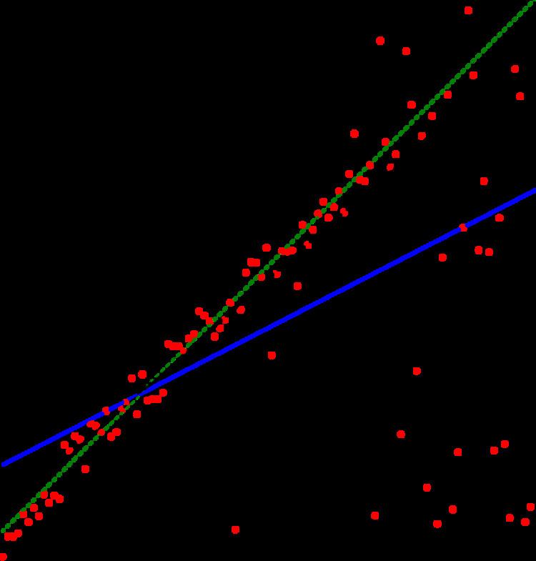
A centerpoint of a point set in a Euclidean space is a point such that any half-space containing the centerpoint also contains a constant fraction of the input points. For d -dimensional spaces, the optimal fraction that can be achieved is always at least 1 / ( d + 1 ) . Parametric-search based algorithms for constructing two-dimensional centerpoints were later improved to linear time using other algorithmic techniques. However, this improvement does not extend to higher dimensions. In three dimensions, parametric search can be used to find centerpoints in time O ( n 2 log 4 n ) (Cole 1987).Parametric search can be used as the basis for an O ( n log n ) time algorithm for the Theil–Sen estimator, a method in robust statistics for fitting a line to a set of points that is much less sensitive to outliers than simple linear regression (Cole et al. 1989).In computer graphics, the ray shooting problem (determining the first object in a scene that is intersected by a given line of sight or light beam) can be solved by combining parametric search with a data structure for a simpler problem, testing whether any of a given set of obstacles occludes a given ray (Agarwal & Matoušek 1993).The biggest stick problem involves finding the longest line segment that lies entirely within a given polygon. It can be solved in time O ( n 8 / 5 + ϵ ) , for n -sided polygons and any ϵ > 0 , using an algorithm based on parametric search (Agarwal, Sharir & Toledo 1994).The annulus that contains a given point set and has the smallest possible width (difference between inner and outer radii) can be used as a measure of the roundness of the point set. Again, this problem can be solved in time O ( n 8 / 5 + ϵ ) , for n -sided polygons and any ϵ > 0 , using an algorithm based on parametric search (Agarwal, Sharir & Toledo 1994).The Hausdorff distance between translates of two polygons, with the translation chosen to minimize the distance, can be found using parametric search in time O ( ( m n ) 2 log 3 m n ) , where m and n are the numbers of sides of the polygons (Agarwal, Sharir & Toledo 1994).The Fréchet distance between two polygonal chains can be computed using parametric search in time O ( m n log m n ) , where m and n are the numbers of segments of the curves (Alt & Godau 1995).For n points in the Euclidean plane, moving at constant velocities, the time at which the points obtain the smallest diameter (and the diameter at that time) can be found using a variation of Cole's technique in time O ( n log 2 n ) . Parametric search can also be used for other similar problems of finding the time at which some measure of a set of moving points obtains its minimum value, for measures including the size of the minimum enclosing ball or the weight of the maximum spanning tree (Fernández-Baca 2001).