Oort constants

Historical significance and background

By the 1920s, a large fraction of the astronomical community had recognized that some of the diffuse, cloud-like objects, or nebulae, seen in the night sky were collections of stars located beyond our own, local collection of star clusters. These galaxies had diverse morphologies, ranging from ellipsoids to disks. The concentrated band of starlight that is the visible signature of the Milky Way was indicative of a disk structure for our galaxy; however, our location within our galaxy made structural determinations from observations difficult.

Classical mechanics predicted that a collection of stars could be supported against gravitational collapse by either random velocities of the stars or their rotation about its center of mass. For a disk-shaped collection, the support should be mainly rotational. Depending on the mass density, or distribution of the mass in the disk, the rotation velocity may be different at each radius from the center of the disk to the outer edge. A plot of these rotational velocities against the radii at which they are measured is called a rotation curve. For external disk galaxies, one can measure the rotation curve by observing the Doppler shifts of spectral features measured along different galactic radii, since one side of the galaxy will be moving towards our line of sight and one side away. However, our position in the Galactic midplane of the Milky Way, where dust in molecular clouds obscures most optical light in many directions, made obtaining our own rotation curve technically difficult until the discovery of the 21 cm hydrogen line in the 1930s.

To confirm the rotation of our galaxy prior to this, in 1927 Jan Oort derived a way to measure the Galactic rotation from just a small fraction of stars in the local neighborhood. As described below, the values he found for A and B proved not only that the Galaxy was rotating but also that it rotates differentially, or as a fluid rather than a solid body.

Derivation

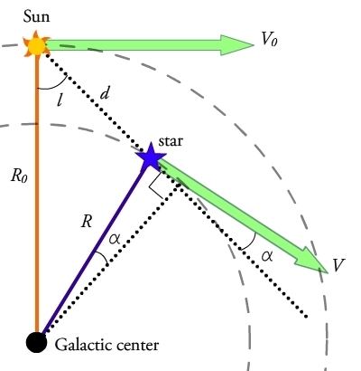
Consider a star in the midplane of the Galactic disk with Galactic longitude l at a distance d from the Sun. Assume that both the star and the Sun have circular orbits around the center of the Galaxy at radii of R and R 0 from the galactic center and rotational velocities of V and V 0 , respectively. The motion of the star along our line of sight, or radial velocity, and motion of the star across the plane of the sky, or transverse velocity, as observed from the position of the Sun are then:

With the assumption of circular motion, the rotational velocity is related to the angular velocity by v = Ω r and we can substitute this into the velocity expressions:

From the geometry in Figure 1, one can see that the triangles formed between the galactic center, the Sun, and the star share a side or portions of sides, so the following relationships hold and substitutions can be made:

and with these we get

To put these expressions only in terms of the known quantities l and d , we take a Taylor expansion of Ω − Ω 0 about R 0 .

Additionally, we take advantage of the assumption that the stars used for this analysis are local, i.e. R − R 0 is small, and the distance d to the star is smaller than R or R 0 , then

So:

Using the sine and cosine half angle formulae, these velocities may be rewritten as:

Writing the velocities in terms of our known quantities and two coefficients A and B yields:

where

At this stage, the observable velocities are related to these coefficients and the position of the star. It is now possible to relate these coefficients to the rotation properties of the galaxy. For a star in a circular orbit, we can express the derivative of the angular velocity with respect to radius in terms of the rotation velocity and radius and evaluate this at the location of the Sun:

so

A is the Oort constant describing the shearing motion and B is the Oort constant describing the rotation of the Galaxy. As described below, one can measure A and B from plotting these velocities, measured for many stars, against the galactic longitudes of these stars.

Measurements

As mentioned in an intermediate step in the derivation above:

Therefore, we can write the Oort constants A and B as:

Thus, the Oort constants can be expressed in terms of the radial and transverse velocities, distances, and galactic longitudes of objects in our Galaxy - all of which are, in principle, observable quantities.

However, there are a number of complications. The simple derivation above assumed that both the Sun and the object in question are traveling on circular orbits about the Galactic center. This is not true for the Sun (the Sun's velocity relative to the local standard of rest is approximately 13.4 km/s), and not necessarily true for other objects in the Milky Way either. The derivation also implicitly assumes that the gravitational potential of the Milky Way is axisymmetric and always directed towards the center. This ignores the effects of spiral arms and the Galaxy's bar. Finally, both transverse velocity and distance are notoriously difficult to measure for objects which are not relatively nearby.

Since the non-circular component of the Sun's velocity is known, it can be subtracted out from our observations to compensate. We do not know, however, the non-circular components of the velocity of each individual star we observe, so they cannot be compensated for in this way. But, if we plot transverse velocity divided by distance against galactic longitude for a large sample of stars, we know from the equations above that they will follow a sine function. The non-circular velocities will introduce scatter around this line, but with a large enough sample the true function can be fit for and the values of the Oort constants measured, as shown in figure 2. A is simply the amplitude of the sinusoid and B is the vertical offset from zero. Measuring transverse velocities and distances accurately and without biases remains challenging, though, and sets of derived values for A and B frequently disagree.

Most methods of measuring A and B are fundamentally similar, following the above patterns. The major differences usually lie in what sorts of objects are used and details of how distance or proper motion are measured. Oort, in his original 1927 paper deriving the constants, obtained A = 31.0 ± 3.7 km s⁻¹ kpc⁻¹. He did not explicitly obtain a value for B , but from his conclusion that the Galaxy was nearly in Keplerian rotation (as in example 2 below), we can presume he would have gotten a value of around -10 km s⁻¹ kpc⁻¹. These differ significantly from modern values, which is indicative of the difficulty of measuring these constants. Measurements of A and B since that time have varied widely; in 1964 the IAU adopted A = 15 km s⁻¹ kpc⁻¹ and B = -10 km s⁻¹ kpc⁻¹ as standard values. Although more recent measurements continue to vary, they tend to lie near these values.

The Hipparcos satellite, launched in 1989, was the first space-based astrometric mission, and its precise measurements of parallax and proper motion have enabled much better measurements of the Oort constants. In 1997 Hipparcos data was used to derive the values A = 14.82 ± 0.84 km s⁻¹ kpc⁻¹ and B = -12.37 ± 0.64 km s⁻¹ kpc⁻¹; these measurements are probably among the most reliable available. The Gaia spacecraft, planned for launch in 2012, is an updated successor to Hipparcos; when it comes online the quality of available data should allow new levels of accuracy in measuring the Oort constants.

Meaning

The Oort constants can greatly enlighten one as to how the Galaxy rotates. As one can see A and B are both functions of the Sun's orbital velocity as well as the first derivative of the Sun's velocity. As a result, A describes the shearing motion in the disk surrounding the Sun, while B describes the angular momentum gradient in the solar neighborhood, also referred to as vorticity.

To illuminate this point, one can look at three examples that describe how stars and gas orbit within the Galaxy giving intuition as to the meaning of A and B . These three examples are solid body rotation, Keplerian rotation and constant rotation over different annuli. These three types of rotation are plotted as a function of radius ( R ), and are shown in Figure 3 as the green, blue and red curves respectively. The grey curve is approximately the rotation curve of the Milky Way.

Solid body rotation

To begin, let one assume that the rotation of the Milky Way can be described by solid body rotation, as shown by the green curve in Figure 3. Solid body rotation assumes that the entire system is moving as a rigid body with no differential rotation. This results in a constant angular velocity, Ω , which is independent of R . Following this we can see that velocity scales linearly with R , v ∝ r , thus

Using the two Oort constant identities, one then can determine what the A and B constants would be,

This demonstrates that in solid body rotation, there is no shear motion, i.e. A = 0 , and the vorticity is just the angular rotation, B = − Ω . This is what one would expect because there is no difference in orbital velocity as radius increases, thus no stress between the annuli. Also, in solid body rotation, the only rotation is about the center, so it is reasonable that the resulting vorticity in the system is described by the only rotation in the system. One can actually measure and find that is non-zero ( A = 14 km s⁻¹ kpc⁻¹.). Thus the galaxy does not rotate as a solid body in our local neighborhood, but may in the inner regions of the Galaxy.

Keplerian rotation

The second illuminating example is to assume that the orbits in the local neighborhood follow a Keplerian orbit, as shown by the blue line in Figure 3. The orbital motion in a Keplerian orbit is described by,

where G is the Gravitational Constant, and M is the mass enclosed within radius r . The derivative of the velocity with respect to the radius is,

The Oort constants can then be written as follows,

For values of Solar velocity, V 0 = 218 km/s, and radius to the Galactic center, R 0 = 8 kpc, the Oort's constants are A = 20 km s⁻¹ kpc⁻¹, and B = − 7 km s⁻¹ kpc⁻¹. However, the observed values are A = 14 km s⁻¹ kpc⁻¹ and B = − 12 km s⁻¹ kpc⁻¹. Thus, Keplerian rotation is not the best description the Milky Way rotation. Furthermore, although this example does not describe the local rotation, it can be thought of as the limiting case that describes the minimum velocity an object can have in a stable orbit.

Flat rotation curve

The final example is to assume that the rotation curve of the Galaxy is flat, i.e. v is constant and independent of radius, r . The rotation velocity is in between that of a solid body and of Keplerian rotation, and is the red dottedline in Figure 3. With a constant velocity, it follows that the radial derivative of v is 0,

and therefore the Oort constants are,

Using the local velocity and radius given in the last example, one finds A = 13.6 km s⁻¹ kpc⁻¹ and B = − 13.6 km s⁻¹ kpc⁻¹. This is remarkably close to the actual measured Oort constants and tells us that the solar neighborhood is roughly rotating with the same linear velocity.

What one should take away from these three examples, is that with a remarkably simple model, the rotation of the Milky Way can be described by these two constants. The first two examples are used as constraints to the Galactic rotation, for they show the fastest and slowest the Galaxy can rotate at a given radius. The flat rotation curve serves as an intermediate step between the two rotation curves, and in fact gives the most reasonable Oort constants as compared to current measurements.

Uses

One of the major uses of the Oort constants is to calibrate the galactic rotation curve. A relative curve can be derived from studying the motions of gas clouds in the Milky Way, but to calibrate the actual absolute speeds involved requires knowledge of V₀. We know that:

Since R₀ can be determined by other means (such as by carefully tracking the motions of stars near the Milky Way's central supermassive black hole), knowing A and B allows us to determine V₀.

It can also be shown that the mass density ρ R can be given by:

So the Oort constants can tell us something about the mass density at a given radius in the disk. They are also useful to constrain mass distribution models for the Galaxy. As well, in the epicyclic approximation for nearly circular stellar orbits in a disk, the epicyclic frequency κ is given by κ 2 = − 4 B Ω , where Ω is the angular velocity. Therefore, the Oort constants can tell us a great deal about motions in the galaxy.