
Median No simple closed form | ||
 | ||
Parameters m o r μ >= 0.5 {\displaystyle m\ or\ \mu >=0.5} shape (real) Ω o r ω > 0 {\displaystyle \Omega \ or\ \omega >0} spread (real) Support x > 0 {\displaystyle x>0\!} PDF 2 m m Γ ( m ) Ω m x 2 m − 1 exp ( − m Ω x 2 ) {\displaystyle {\frac {2m^{m}}{\Gamma (m)\Omega ^{m}}}x^{2m-1}\exp \left(-{\frac {m}{\Omega }}x^{2}\right)} CDF γ ( m , m Ω x 2 ) Γ ( m ) {\displaystyle {\frac {\gamma \left(m,{\frac {m}{\Omega }}x^{2}\right)}{\Gamma (m)}}} Mean Γ ( m + 1 2 ) Γ ( m ) ( Ω m ) 1 / 2 {\displaystyle {\frac {\Gamma (m+{\frac {1}{2}})}{\Gamma (m)}}\left({\frac {\Omega }{m}}\right)^{1/2}} | ||
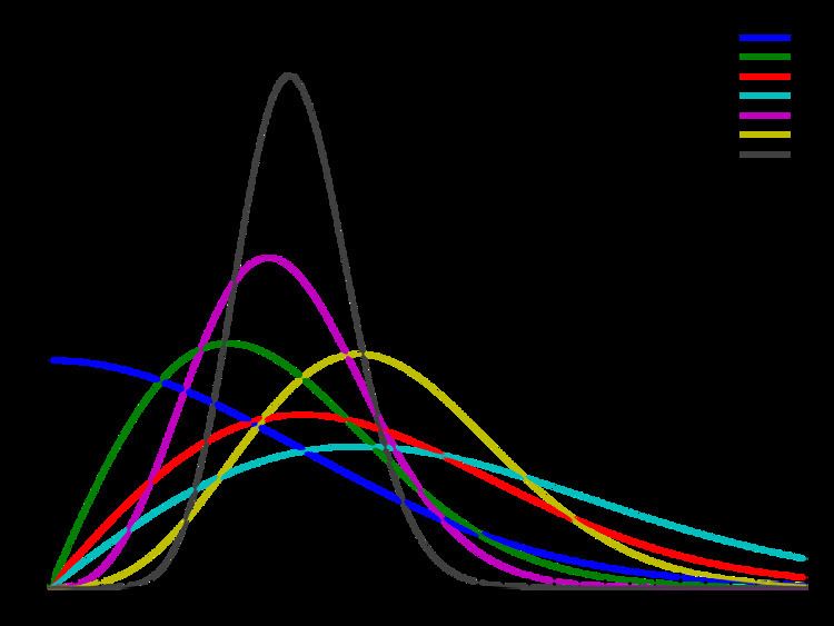
The Nakagami distribution or the Nakagami-m distribution is a probability distribution related to the gamma distribution. It has two parameters: a shape parameter
Contents
Characterization
Its probability density function (pdf) is
Its cumulative distribution function is
where P is the incomplete gamma function (regularized).
Differential equation
Parameter estimation
The parameters
and
An alternative way of fitting the distribution is to re-parametrize
and
It is reported by authors that modelling data with Nakagami distribution and estimating parameters by above mention method results in better performance for low data regime compared to moments based methods.
Generation
The Nakagami distribution is related to the gamma distribution. In particular, given a random variable
Alternatively, the Nakagami distribution
But it should be noted that for a Chi-distribution, the degrees of freedom
Finally, there is also a more efficient generation method using efficient rejection-sampling.
History and applications
The Nakagami distribution is relatively new, being first proposed in 1960. It has been used to model attenuation of wireless signals traversing multiple paths.
Related distributions
"The radius around the true mean in a bivariate normal random variable, re-written in polar coordinates (radius and angle), follows a Hoyt distribution. Equivalently, the modulus of a complex normal random variable does."