
 | ||
Multidimensional Multirate systems find applications in image compression and coding. Several applications such as conversion between progressive video signals require usage of multidimensional multirate systems. In multidimensional multirate systems, the basic building blocks are decimation matrix (M), expansion matrix(L) and Multidimensional digital filters. The decimation and expansion matrices have dimension of D x D, where D represents the dimension. To extend the one dimensional (1-D) multirate results, there are two different ways which are based on the structure of decimation and expansion matrices. If these matrices are diagonal, separable approaches can be used, which are separable operations in each dimension. Although separable approaches might serve less complexity, non-separable methods, with non-diagonal expansion and decimation matrices, provide much better performance. The difficult part in non-separable methods is to create results in MD case by extend the 1-D case. Polyphase decomposition and maximally decimated reconstruction systems are already carried out.
Contents
- Basic Building Blocks of MD Multirate Systems
- MD Multirate Filters Derived from 1 D Filters
- MD Maximally Decimated Filter Banks
- References
MD decimation / interpolation filters derived from 1-D filters and maximally decimated filter banks are widely used and constitute important steps in the design of multidimensional multirate systems.
Basic Building Blocks of MD Multirate Systems
Decimation and interpolation are necessary steps to create multidimensional multirate systems. In the one dimensional system, decimation and interpolation can be seen in the figure.
Theoretically, explanations of decimation and interpolation are:
• Decimation (Down-sampling):
The M times decimated version of x(n) is defined as y(n)= x(Mn), where M is a nonsingular integer matrix called decimation matrix.
In the frequency domain, relation becomes
where
Above expression changes in multidimensional case, In 2-D case M matrix becomes 2x2 and the region becomes parallel-ogram which is defined as:
• Expansion (Up-sampling):
The L times up sampled version of x(n) defined as Y(n)= x(L−1 . n), where n is in the range of lattice generated by L which is L*m. The matrix L is called expansion matrix.
MD Multirate Filters Derived from 1-D Filters
In the one dimensional systems, the decimator term is used for decimation filter and expander term is used for interpolation filter. The decimator filters generally have the range of [-π / M, π / M], where M is decimation matrix. In the multidimensional decimation and expansion, the passband changes to:
where x in the range of [-1, 1)D
When M matrix is not diagonal, the filters are not separable. The complexity of non-separable filters increase with increasing number of dimension. Design procedure and example:
- Design a one dimensional low pass filter
P ( w ) , whose response will be similar to the figure of 1-D frequency response . - Construct the separable MD filter
h ( s ) ( n ) fromp ( n ) , which is constructed from one dimensional low pass filterP ( w ) . - Decimate
h ( s ) ( n ) by M and scale it to findh ( n ) .
In detail, By using prototype filter
for k=D-1, where D represents number of dimensions:
This is separable low pass filter and its impulse response will be;
where k=D-1, where D represents number of dimensions:
Now, considering
we get:
This process basically shows how to derive MD multirate filter from 1-D filter.
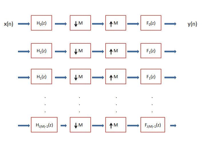
MD Maximally Decimated Filter Banks
When the number of channel is equal to J(M), this is called a maximally decimated filter bank. To analyze filter banks, polyphase decomposition is used.
Polyphase decomposition:
The polyphase components of x(n) with respect to the given M,
Where ki can takes the values of k0,k1,…kJ(M)-1. In the z domain,
where