Maxwell–Boltzmann statistics

Applications

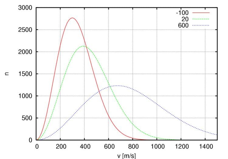
Maxwell–Boltzmann statistics may be used to derive the Maxwell–Boltzmann distribution (for an ideal gas of classical particles in a three-dimensional box). However, they apply to other situations as well. Maxwell–Boltzmann statistics can be used to extend that distribution to particles with a different energy–momentum relation, such as relativistic particles (Maxwell–Jüttner distribution). In addition, hypothetical situations can be considered, such as particles in a box with different numbers of dimensions (four-dimensional, two-dimensional, etc.).

Limits of applicability

Maxwell–Boltzmann statistics are often described as the statistics of "distinguishable" classical particles. In other words, the configuration of particle A in state 1 and particle B in state 2 is different from the case in which particle B is in state 1 and particle A is in state 2. This assumption leads to the proper (Boltzmann) statistics of particles in the energy states, but yields non-physical results for the entropy, as embodied in the Gibbs paradox.

At the same time, there are no real particles which have the characteristics required by Maxwell–Boltzmann statistics. Indeed, the Gibbs paradox is resolved if we treat all particles of a certain type (e.g., electrons, protons, etc.) as indistinguishable, and this assumption can be justified in the context of quantum mechanics. Once this assumption is made, the particle statistics change. Quantum particles are either bosons (following instead Bose–Einstein statistics) or fermions (subject to the Pauli exclusion principle, following instead Fermi–Dirac statistics). Both of these quantum statistics approach the Maxwell–Boltzmann statistics in the limit of high temperature and low particle density, without the need for any ad hoc assumptions. The Fermi–Dirac and Bose–Einstein statistics give the energy level occupation as:

It can be seen that the condition under which the Maxwell–Boltzmann statistics are valid is when

where ε m i n is the lowest (minimum) value of ε i .

Maxwell–Boltzmann statistics are particularly useful for studying gases that are not very dense. Note, however, that all of these statistics assume that the particles are non-interacting and have static energy states.

Derivations of Maxwell–Boltzmann statistics

Maxwell–Boltzmann statistics can be derived in various statistical mechanical thermodynamic ensembles:

In each case it is necessary to assume that the particles are non-interacting, and that multiple particles can occupy the same state and do so independently.

Derivation from microcanonical ensemble

Suppose we have a container with a huge number of very small particles all with identical physical characteristics (such as mass, charge, etc.). Let's refer to this as the system. Assume that though the particles have identical properties, they are distinguishable. For example, we might identify each particle by continually observing their trajectories, or by placing a marking on each one, e.g., drawing a different number on each one as is done with lottery balls.

The particles are moving inside that container in all directions with great speed. Because the particles are speeding around, they possess some energy. The Maxwell–Boltzmann distribution is a mathematical function that speaks about how many particles in the container have a certain energy.

In general, there may be many particles with the same amount of energy ε . Let the number of particles with the same energy ε 1 be N 1 , the number of particles possessing another energy ε 2 be N 2 , and so forth for all the possible energies { ε i | i=1,2,3,...}. To describe this situation, we say that N i is the occupation number of the energy level i . If we know all the occupation numbers { N i | i=1,2,3,...}, then we know the total energy of the system. However, because we can distinguish between which particles are occupying each energy level, the set of occupation numbers { N i | i=1,2,3,...} does not completely describe the state of the system. To completely describe the state of the system, or the microstate, we must specify exactly which particles are in each energy level. Thus when we count the number of possible states of the system, we must count each and every microstate, and not just the possible sets of occupation numbers.

To begin with, let's ignore the degeneracy problem: assume that there is only one way to put N i particles into the energy level i  . What follows next is a bit of combinatorial thinking which has little to do in accurately describing the reservoir of particles.

The number of different ways of performing an ordered selection of one single object from N objects is obviously N. The number of different ways of selecting two objects from N objects, in a particular order, is thus N(N − 1) and that of selecting n objects in a particular order is seen to be N!/(N − n)!. It is divided by the number of permutations, n!, if order does not matter. The binomial coefficient, N!/(n!(N − n)!), is, thus, the number of ways to pick n objects from N . If we now have a set of boxes labelled a, b, c, d, e, ..., k, then the number of ways of selecting N_a objects from a total of N objects and placing them in box a, then selecting N_b objects from the remaining N − N_a objects and placing them in box b, then selecting N_c objects from the remaining N − N_a − N_b objects and placing them in box c, and continuing until no object is left outside is

and because not even a single object is to be left outside the boxes, implies that the sum made of the terms N_a, N_b, N_c, N_d, N_e, ..., N_k must equal N, thus the term (N - N_a - N_b - N_c - ... - N_l - N_k)! in the relation above evaluates to 0!. (0!=1) which makes possible to write down that relation as

This is just the multinomial coefficient, the number of ways of arranging N items into k boxes, the i-th box holding N_i items, ignoring the permutation of items in each box.

Now going back to the degeneracy problem which characterizes the reservoir of particles. If the i-th box has a "degeneracy" of g i , that is, it has g i "sub-boxes", such that any way of filling the i-th box where the number in the sub-boxes is changed is a distinct way of filling the box, then the number of ways of filling the i-th box must be increased by the number of ways of distributing the N i objects in the g i "sub-boxes". The number of ways of placing N i distinguishable objects in g i "sub-boxes" is g i N i (the first object can go into any of the g i boxes, the second object can also go into any of the g i boxes, and so on). Thus the number of ways W that a total of N particles can be classified into energy levels according to their energies, while each level i having g i distinct states such that the i-th level accommodates N i particles is:

This is the form for W first derived by Boltzmann. Boltzmann's fundamental equation S = k ln ⁡ W relates the thermodynamic entropy S to the number of microstates W, where k is the Boltzmann constant. It was pointed out by Gibbs however, that the above expression for W does not yield an extensive entropy, and is therefore faulty. This problem is known as the Gibbs paradox. The problem is that the particles considered by the above equation are not indistinguishable. In other words, for two particles (A and B) in two energy sublevels the population represented by [A,B] is considered distinct from the population [B,A] while for indistinguishable particles, they are not. If we carry out the argument for indistinguishable particles, we are led to the Bose–Einstein expression for W:

The Maxwell–Boltzmann distribution follows from this Bose–Einstein distribution for temperatures well above absolute zero, implying that g i ≫ 1 . The Maxwell–Boltzmann distribution also requires low density, implying that g i ≫ N i . Under these conditions, we may use Stirling's approximation for the factorial:

to write:

Using the fact that ( 1 + N i / g i ) g i ≈ e N i for g i ≫ N i we can again use Stirlings approximation to write:

This is essentially a division by N! of Boltzmann's original expression for W, and this correction is referred to as correct Boltzmann counting.

We wish to find the N i for which the function W is maximized, while considering the constraint that there is a fixed number of particles ( N = ∑ N i ) and a fixed energy ( E = ∑ N i ε i ) in the container. The maxima of W and ln ⁡ ( W ) are achieved by the same values of N i and, since it is easier to accomplish mathematically, we will maximize the latter function instead. We constrain our solution using Lagrange multipliers forming the function:

Finally

In order to maximize the expression above we apply Fermat's theorem (stationary points), according to which local extrema, if exist, must be at critical points (partial derivatives vanish):

By solving the equations above ( i = 1 … n ) we arrive to an expression for N i :

Substituting this expression for N i into the equation for ln ⁡ W and assuming that N ≫ 1 yields:

or, rearranging:

Boltzmann realized that this is just an expression of the Euler-integrated fundamental equation of thermodynamics. Identifying E as the internal energy, the Euler-integrated fundamental equation states that :

where T is the temperature, P is pressure, V is volume, and μ is the chemical potential. Boltzmann's famous equation S = k ln ⁡ W is the realization that the entropy is proportional to ln ⁡ W with the constant of proportionality being Boltzmann's constant. Using the ideal gas equation of state (PV=NkT), It follows immediately that β = 1 / k T and α = − μ / k T so that the populations may now be written:

Note that the above formula is sometimes written:

where z = exp ⁡ ( μ / k T ) is the absolute activity.

Alternatively, we may use the fact that

to obtain the population numbers as

where Z is the partition function defined by:

In an approximation where ε_i is considered to be a continuous variable, the Thomas-Fermi approximation yields a continuous degeneracy g proportional to ε so that:

which is just the Maxwell-Boltzmann distribution for the energy.

Derivation from canonical ensemble

In the above discussion, the Boltzmann distribution function was obtained via directly analysing the multiplicities of a system. Alternatively, one can make use of the canonical ensemble. In a canonical ensemble, a system is in thermal contact with a reservoir. While energy is free to flow between the system and the reservoir, the reservoir is thought to have infinitely large heat capacity as to maintain constant temperature, T, for the combined system.

In the present context, our system is assumed to have the energy levels ε i with degeneracies g i . As before, we would like to calculate the probability that our system has energy ε i .

If our system is in state s 1 , then there would be a corresponding number of microstates available to the reservoir. Call this number Ω R ( s 1 ) . By assumption, the combined system (of the system we are interested in and the reservoir) is isolated, so all microstates are equally probable. Therefore, for instance, if Ω R ( s 1 ) = 2 Ω R ( s 2 ) , we can conclude that our system is twice as likely to be in state s 1 than s 2 . In general, if P ( s i ) is the probability that our system is in state s i ,

Since the entropy of the reservoir S R = k ln ⁡ Ω R , the above becomes

Next we recall the thermodynamic identity (from the first law of thermodynamics):

In a canonical ensemble, there is no exchange of particles, so the d N R term is zero. Similarly, d V R = 0. This gives

where U R ( s i ) and E ( s i ) denote the energies of the reservoir and the system at s i , respectively. For the second equality we have used the conservation of energy. Substituting into the first equation relating P ( s 1 ) , P ( s 2 ) :

which implies, for any state s of the system

where Z is an appropriately chosen "constant" to make total probability 1. (Z is constant provided that the temperature T is invariant.) It is obvious that

where the index s runs through all microstates of the system. Z is sometimes called the Boltzmann sum over states (or "Zustandsumme" in the original German). If we index the summation via the energy eigenvalues instead of all possible states, degeneracy must be taken into account. The probability of our system having energy ε i is simply the sum of the probabilities of all corresponding microstates:

where, with obvious modification,

this is the same result as before.

Comments on this derivation: