Cost curve

Short-run average variable cost curve (SRAVC)

Average variable cost (which is a short-run concept) is the variable cost (typically labor cost) per unit of output: SRAVC = wL / Q where w is the wage rate, L is the quantity of labor used, and Q is the quantity of output produced. The SRAVC curve plots the short-run average variable cost against the level of output and is typically drawn as U-shaped.

Short-run average total cost curve (SRATC or SRAC)

The average total cost curve is constructed to capture the relation between cost per unit of output and the level of output, ceteris paribus. A perfectly competitive and productively efficient firm organizes its factors of production in such a way that the factors of production is at the lowest point. In the short run, when at least one factor of production is fixed, this occurs at the output level where it has enjoyed all possible average cost gains from increasing production. This is at the minimum point in the diagram on the right.

Short-run total cost is given by

S T C = P K . K + P L . L ,

where P_K is the unit price of using physical capital per unit time, P_L is the unit price of labor per unit time (the wage rate), K is the quantity of physical capital used, and L is the quantity of labor used. From this we obtain short-run average cost, denoted either SATC or SAC, as STC / Q:

SRATC or SRAC = P_KK/Q + P_LL/Q = P_K / AP_K + P_L / AP_L,

where AP_K = Q/K is the average product of capital and AP_L = Q/L is the average product of labor.

Within the graph shown in the figure, The Marginal cost curve, Average Fixed Cost curve and Average Variable cost curve can not start with zero as at quantity zero, these values are not defined.

Short run average cost equals average fixed costs plus average variable costs. Average fixed cost continuously falls as production increases in the short run, because K is fixed in the short run. The shape of the average variable cost curve is directly determined by increasing and then diminishing marginal returns to the variable input (conventionally labor).

Short-run marginal cost curve (SRMC)

A short-run marginal cost curve graphically represents the relation between marginal (i.e., incremental) cost incurred by a firm in the short-run production of a good or service and the quantity of output produced. This curve is constructed to capture the relation between marginal cost and the level of output, holding other variables, like technology and resource prices, constant. The marginal cost curve is usually U-shaped. Marginal cost is relatively high at small quantities of output; then as production increases, marginal cost declines, reaches a minimum value, then rises. The marginal cost is shown in relation to marginal revenue (MR), the incremental amount of sales revenue that an additional unit of the product or service will bring to the firm. This shape of the marginal cost curve is directly attributable to increasing, then decreasing marginal returns (and the law of diminishing marginal returns). Marginal cost equals w/MP_L. For most production processes the marginal product of labor initially rises, reaches a maximum value and then continuously falls as production increases. Thus marginal cost initially falls, reaches a minimum value and then increases. The marginal cost curve intersects both the average variable cost curve and (short-run) average total cost curve at their minimum points. When the marginal cost curve is above an average cost curve the average curve is rising. When the marginal costs curve is below an average curve the average curve is falling. This relation holds regardless of whether the marginal curve is rising or falling.

Long-run marginal cost curve (LRMC)

The long-run marginal cost curve shows for each unit of output the added total cost incurred in the long run, that is, the conceptual period when all factors of production are variable so as minimize long-run average total cost. Stated otherwise, LRMC is the minimum increase in total cost associated with an increase of one unit of output when all inputs are variable.

The long-run marginal cost curve is shaped by returns to scale, a long-run concept, rather than the law of diminishing marginal returns, which is a short-run concept. The long-run marginal cost curve tends to be flatter than its short-run counterpart due to increased input flexibility as to cost minimization. The long-run marginal cost curve intersects the long-run average cost curve at the minimum point of the latter. When long-run marginal costs are below long-run average costs, long-run average costs are falling (as to additional units of output). When long-run marginal costs are above long run average costs, average costs are rising. Long-run marginal cost equals short run marginal-cost at the least-long-run-average-cost level of production. LRMC is the slope of the LR total-cost function.

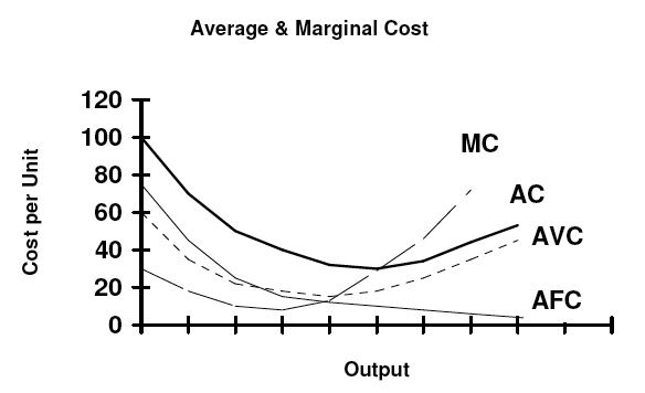
Graphing cost curves together

Cost curves can be combined to provide information about firms. In this diagram for example, firms are assumed to be in a perfectly competitive market. In a perfectly competitive market the price that firms are faced with would be the price at which the marginal cost curve cuts the average cost curve.

Cost curves and production functions

Assuming that factor prices are constant, the production function determines all cost functions. The variable cost curve is the inverted short-run production function or total product curve and its behavior and properties are determined by the production function. Because the production function determines the variable cost function it necessarily determines the shape and properties of marginal cost curve and the average cost curves.

If the firm is a perfect competitor in all input markets, and thus the per-unit prices of all its inputs are unaffected by how much of the inputs the firm purchases, then it can be shown that at a particular level of output, the firm has economies of scale (i.e., is operating in a downward sloping region of the long-run average cost curve) if and only if it has increasing returns to scale. Likewise, it has diseconomies of scale (is operating in an upward sloping region of the long-run average cost curve) if and only if it has decreasing returns to scale, and has neither economies nor diseconomies of scale if it has constant returns to scale. In this case, with perfect competition in the output market the long-run market equilibrium will involve all firms operating at the minimum point of their long-run average cost curves (i.e., at the borderline between economies and diseconomies of scale).

If, however, the firm is not a perfect competitor in the input markets, then the above conclusions are modified. For example, if there are increasing returns to scale in some range of output levels, but the firm is so big in one or more input markets that increasing its purchases of an input drives up the input's per-unit cost, then the firm could have diseconomies of scale in that range of output levels. Conversely, if the firm is able to get bulk discounts of an input, then it could have economies of scale in some range of output levels even if it has decreasing returns in production in that output range.

Relationship between different curves

Total Cost = Fixed Costs (FC) + Variable Costs (VC)

Marginal Cost (MC) = dC/dQ; MC equals the slope of the total cost function and of the variable cost function

Average Total Cost (ATC) = Total Cost/Q

Average Fixed Cost (AFC) = FC/Q

Average Variable Cost (AVC) = VC/Q.

ATC = AFC + AVC

The MC curve is related to the shape of the ATC and AVC curves:

At a level of Q at which the MC curve is above the average total cost or average variable cost curve, the latter curve is rising.

If MC is below average total cost or average variable cost, then the latter curve is falling.

If MC equals average total cost, then average total cost is at its minimum value.

If MC equals average variable cost, then average variable cost is at its minimum value.

Relationship between short run and long run cost curves

Basic: For each quantity of output there is one cost minimizing level of capital and a unique short run average cost curve associated with producing the given quantity.

Each STC curve can be tangent to the LRTC curve at only one point. The STC curve cannot cross (intersect) the LRTC curve. The STC curve can lie wholly “above” the LRTC curve with no tangency point.

One STC curve is tangent to LRTC at the long-run cost minimizing level of production. At the point of tangency LRTC = STC. At all other levels of production STC will exceed LRTC.

Average cost functions are the total cost function divided by the level of output. Therefore, the SATC curveis also tangent to the LRATC curve at the cost-minimizing level of output. At the point of tangency LRATC = SATC. At all other levels of production SATC > LRATC To the left of the point of tangency the firm is using too much capital and fixed costs are too high. To the right of the point of tangency the firm is using too little capital and diminishing returns to labor are causing costs to increase.

The slope of the total cost curves equals marginal cost. Therefore, when STC is tangent to LTC, SMC = LRMC.

At the long run cost minimizing level of output LRTC = STC; LRATC = SATC and LRMC = SMC,.

The long run cost minimizing level of output may be different from minimum SATC,.

With fixed unit costs of inputs, if the production function has constant returns to scale, then at the minimal level of the SATC curve we have SATC = LRATC = SMC = LRMC.

With fixed unit costs of inputs, if the production function has increasing returns to scale, the minimum of the SATC curve is to the right of the point of tangency between the LRAC and the SATC curves. Where LRTC = STC, LRATC = SATC and LRMC = SMC.

With fixed unit costs of inputs and decreasing returns the minimum of the SATC curve is to the left of the point of tangency between LRAC and SATC. Where LRTC = STC, LRATC = SATC and LRMC = SMC.

With fixed unit input costs, a firm that is experiencing increasing (decreasing) returns to scale and is producing at its minimum SAC can always reduce average cost in the long run by expanding (reducing) the use of the fixed input.

LRATC will always equal to or be less than SATC.

If production process is exhibiting constant returns to scale then minimum SRAC equals minimum long run average cost. The LRAC and SRAC intersect at their common minimum values. Thus under constant returns to scale SRMC = LRMC = LRAC = SRAC .

If the production process is experiencing decreasing or increasing, minimum short run average cost does not equal minimum long run average cost. If increasing returns to scale exist long run minimum will occur at a lower level of output than SRAC. This is because there are economies of scale that have not been exploited so in the long run a firm could always produce a quantity at a price lower than minimum short run average cost simply by using a larger plant.

With decreasing returns, minimum SRAC occurs at a lower production level than minimum LRAC because a firm could reduce average costs by simply decreasing the size or its operations.

The minimum of a SRAC occurs when the slope is zero. Thus the points of tangency between the U-shaped LRAC curve and the minimum of the SRAC curve would coincide only with that portion of the LRAC curve exhibiting constant economies of scale. For increasing returns to scale the point of tangency between the LRAC and the SRAC would have to occur at a level of output below level associated with the minimum of the SRAC curve.

These statements assume that the firm is using the optimal level of capital for the quantity produced. If not, then the SRAC curve would lie "wholly above" the LRAC and would not be tangent at any point.

U-shaped curves

Both the SRAC and LRAC curves are typically expressed as U-shaped. However, the shapes of the curves are not due to the same factors. For the short run curve the initial downward slope is largely due to declining average fixed costs. Increasing returns to the variable input at low levels of production also play a role, while the upward slope is due to diminishing marginal returns to the variable input. With the long run curve the shape by definition reflects economies and diseconomies of scale. At low levels of production long run production functions generally exhibit increasing returns to scale, which, for firms that are perfect competitors in input markets, means that the long run average cost is falling; the upward slope of the long run average cost function at higher levels of output is due to decreasing returns to scale at those output levels.

Cost curves in reality

Evidence shows that cost curves are not typically U-shaped. In a survey by Wilford J. Eiteman and Glenn E. Guthrie in 1952 managers of 334 companies were shown a number of different cost curves, and asked to specify which one best represented the company’s cost curve. 95% of managers responding to the survey reported cost curves with constant or falling costs.

Alan Blinder, former vice president of the American Economics Association, conducted the same type of survey in 1998, which involved 200 US firms in a sample that should be representative of the US economy at large. He found that about 40% of firms reported falling variable or marginal cost, and 48.4% reported constant marginal/variable cost.