
 | ||
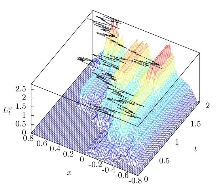
In the mathematical theory of stochastic processes, local time is a stochastic process associated with diffusion processes such as Brownian motion, that characterizes the amount of time a particle has spent at a given level. Local time appears in various stochastic integration formulas, such as Tanaka's formula, if the integrand is not sufficiently smooth. It is also studied in statistical mechanics in the context of random fields.
Contents
Formal definition
For a real valued diffusion process
where
which explains why it is called the local time of
Tanaka's formula
Tanaka's formula provides a definition of local time for an arbitrary continuous semimartingale
A more general form was proven independently by Meyer and Wang; the formula extends Itô's lemma for twice differentiable functions to a more general class of functions. If
where
If
Tanaka's formula provides the explicit Doob–Meyer decomposition for the one-dimensional reflecting Brownian motion,
Ray–Knight theorems
The field of local times
In general Ray–Knight type theorems of the first kind consider the field Lt at a hitting time of the underlying process, whilst theorems of the second kind are in terms of a stopping time at which the field of local times first exceeds a given value.
First Ray–Knight theorem
Let (Bt)t ≥ 0 be a one-dimensional Brownian motion started from B0 = a > 0, and (Wt)t≥0 be a standard two-dimensional Brownian motion W0 = 0 ∈ R2. Define the stopping time at which B first hits the origin,
where (Lt)t ≥ 0 is the field of local times of (Bt)t ≥ 0, and equality is in distribution on C[0, a]. The process |Wx|2 is known as the squared Bessel process.
Second Ray–Knight theorem
Let (Bt)t ≥ 0 be a standard one-dimensional Brownian motion B0 = 0 ∈ R, and let (Lt)t ≥ 0 be the associated field of local times. Let Ta be the first time at which the local time at zero exceeds a > 0
Let (Wt)t ≥ 0 be an independent one-dimensional Brownian motion started from W0 = 0, then
Equivalently, the process
Generalized Ray–Knight theorems
Results of Ray–Knight type for more general stochastic processes have been intensively studied, and analogue statements of both (1) and (2) are known for strongly symmetric Markov processes.