K nearest neighbors algorithm

Statistical setting

Suppose we have pairs ( X , Y ) , ( X 1 , Y 1 ) , … , ( X n , Y n ) taking values in R d × { 1 , 2 } , where Y is the class label of X, so that X | Y = r ∼ P r for r = 1 , 2 (and probability distributions P r ). Given some norm ∥ ⋅ ∥ on R d and a point x ∈ R d , let ( X ( 1 ) , Y ( 1 ) ) , … , ( X ( n ) , Y ( n ) ) be a reordering of the training data such that ∥ X ( 1 ) − x ∥ ≤ ⋯ ≤ ∥ X ( n ) − x ∥ .

Algorithm

The training examples are vectors in a multidimensional feature space, each with a class label. The training phase of the algorithm consists only of storing the feature vectors and class labels of the training samples.

In the classification phase, k is a user-defined constant, and an unlabeled vector (a query or test point) is classified by assigning the label which is most frequent among the k training samples nearest to that query point.

A commonly used distance metric for continuous variables is Euclidean distance. For discrete variables, such as for text classification, another metric can be used, such as the overlap metric (or Hamming distance). In the context of gene expression microarray data, for example, k-NN has also been employed with correlation coefficients such as Pearson and Spearman. Often, the classification accuracy of k-NN can be improved significantly if the distance metric is learned with specialized algorithms such as Large Margin Nearest Neighbor or Neighbourhood components analysis.

A drawback of the basic "majority voting" classification occurs when the class distribution is skewed. That is, examples of a more frequent class tend to dominate the prediction of the new example, because they tend to be common among the k nearest neighbors due to their large number. One way to overcome this problem is to weight the classification, taking into account the distance from the test point to each of its k nearest neighbors. The class (or value, in regression problems) of each of the k nearest points is multiplied by a weight proportional to the inverse of the distance from that point to the test point. Another way to overcome skew is by abstraction in data representation. For example, in a self-organizing map (SOM), each node is a representative (a center) of a cluster of similar points, regardless of their density in the original training data. K-NN can then be applied to the SOM.

Parameter selection

The best choice of k depends upon the data; generally, larger values of k reduce the effect of noise on the classification, but make boundaries between classes less distinct. A good k can be selected by various heuristic techniques (see hyperparameter optimization). The special case where the class is predicted to be the class of the closest training sample (i.e. when k = 1) is called the nearest neighbor algorithm.

The accuracy of the k-NN algorithm can be severely degraded by the presence of noisy or irrelevant features, or if the feature scales are not consistent with their importance. Much research effort has been put into selecting or scaling features to improve classification. A particularly popular approach is the use of evolutionary algorithms to optimize feature scaling. Another popular approach is to scale features by the mutual information of the training data with the training classes.

In binary (two class) classification problems, it is helpful to choose k to be an odd number as this avoids tied votes. One popular way of choosing the empirically optimal k in this setting is via bootstrap method.

The 1-nearest neighbour classifier

The most intuitive nearest neighbour type classifier is the one nearest neighbour classifier that assigns a point x to the class of its closest neighbour in the feature space, that is C n 1 n n ( x ) = Y ( 1 ) .

As the size of training data set approaches infinity, the one nearest neighbour classifier guarantees an error rate of no worse than twice the Bayes error rate (the minimum achievable error rate given the distribution of the data).

The weighted nearest neighbour classifier

The k-nearest neighbour classifier can be viewed as assigning the k nearest neighbours a weight 1 / k and all others 0 weight. This can be generalised to weighted nearest neighbour classifiers. That is, where the ith nearest neighbour is assigned a weight w n i , with ∑ i = 1 n w n i = 1 . An analogous result on the strong consistency of weighted nearest neighbour classifiers also holds.

Let C n w n n denote the weighted nearest classifier with weights { w n i } i = 1 n . Subject to regularity conditions on to class distributions the excess risk has the following asymptotic expansion

for constants B 1 and B 2 where s n 2 = ∑ i = 1 n w n i 2 and t n = n − 2 / d ∑ i = 1 n w n i { i 1 + 2 / d − ( i − 1 ) 1 + 2 / d } .

The optimal weighting scheme { w n i ∗ } i = 1 n , that balances the two terms in the display above, is given as follows: set k ∗ = ⌊ B n 4 d + 4 ⌋ ,

With optimal weights the dominant term in the asymptotic expansion of the excess risk is O ( n − 4 d + 4 ) . Similar results are true when using a bagged nearest neighbour classifier.

Properties

k-NN is a special case of a variable-bandwidth, kernel density "balloon" estimator with a uniform kernel.

The naive version of the algorithm is easy to implement by computing the distances from the test example to all stored examples, but it is computationally intensive for large training sets. Using an appropriate nearest neighbor search algorithm makes k-NN computationally tractable even for large data sets. Many nearest neighbor search algorithms have been proposed over the years; these generally seek to reduce the number of distance evaluations actually performed.

k-NN has some strong consistency results. As the amount of data approaches infinity, the two-class k-NN algorithm is guaranteed to yield an error rate no worse than twice the Bayes error rate (the minimum achievable error rate given the distribution of the data). Various improvements to the k-NN speed are possible by using proximity graphs.

For multi-class k-NN classification, Cover and Hart (1967) prove an upper bound error rate of

R ∗   ≤   R k N N   ≤   R ∗ ( 2 − M R ∗ / ( M − 1 ) )

where R ∗ is the Bayes error rate (which is the minimal error rate possible), R k N N is the k-NN error rate, and M is the number of classes in the problem. For M =2 and as the Bayesian error rate R ∗ approaches zero, this limit reduces to "not more than twice the Bayesian error rate".

Error rates

There are many results on the error rate of the k nearest neighbour classifiers. The k-nearest neighbour classifier is strongly (that is for any joint distribution on ( X , Y ) ) consistent provided k := k n diverges and k n / n converges to zero as n → ∞ .

Let C n k n n denote the k nearest neighbour classifier based on a training set of size n. Under certain regularity conditions, the excess risk yields the following asymptotic expansion

for some constants B 1 and B 2 .

The choice k ∗ = ⌊ B n 4 d + 4 ⌋ offers a trade off between the two terms in the above display, for which the k ∗ -nearest neighbour error converges to the Bayes error at the optimal (minimax) rate O ( n − 4 d + 4 ) .

Metric learning

The K-nearest neighbor classification performance can often be significantly improved through (supervised) metric learning. Popular algorithms are neighbourhood components analysis and large margin nearest neighbor. Supervised metric learning algorithms use the label information to learn a new metric or pseudo-metric.

Feature extraction

When the input data to an algorithm is too large to be processed and it is suspected to be redundant (e.g. the same measurement in both feet and meters) then the input data will be transformed into a reduced representation set of features (also named features vector). Transforming the input data into the set of features is called feature extraction. If the features extracted are carefully chosen it is expected that the features set will extract the relevant information from the input data in order to perform the desired task using this reduced representation instead of the full size input. Feature extraction is performed on raw data prior to applying k-NN algorithm on the transformed data in feature space.

An example of a typical computer vision computation pipeline for face recognition using k-NN including feature extraction and dimension reduction pre-processing steps (usually implemented with OpenCV):

1. Haar face detection
2. Mean-shift tracking analysis
3. PCA or Fisher LDA projection into feature space, followed by k-NN classification

Dimension reduction

For high-dimensional data (e.g., with number of dimensions more than 10) dimension reduction is usually performed prior to applying the k-NN algorithm in order to avoid the effects of the curse of dimensionality.

The curse of dimensionality in the k-NN context basically means that Euclidean distance is unhelpful in high dimensions because all vectors are almost equidistant to the search query vector (imagine multiple points lying more or less on a circle with the query point at the center; the distance from the query to all data points in the search space is almost the same).

Feature extraction and dimension reduction can be combined in one step using principal component analysis (PCA), linear discriminant analysis (LDA), or canonical correlation analysis (CCA) techniques as a pre-processing step, followed by clustering by k-NN on feature vectors in reduced-dimension space. In machine learning this process is also called low-dimensional embedding.

For very-high-dimensional datasets (e.g. when performing a similarity search on live video streams, DNA data or high-dimensional time series) running a fast approximate k-NN search using locality sensitive hashing, "random projections", "sketches" or other high-dimensional similarity search techniques from the VLDB toolbox might be the only feasible option.

Decision boundary

Nearest neighbor rules in effect implicitly compute the decision boundary. It is also possible to compute the decision boundary explicitly, and to do so efficiently, so that the computational complexity is a function of the boundary complexity.

Data reduction

Data reduction is one of the most important problems for work with huge data sets. Usually, only some of the data points are needed for accurate classification. Those data are called the prototypes and can be found as follows:

1. Select the class-outliers, that is, training data that are classified incorrectly by k-NN (for a given k)
2. Separate the rest of the data into two sets: (i) the prototypes that are used for the classification decisions and (ii) the absorbed points that can be correctly classified by k-NN using prototypes. The absorbed points can then be removed from the training set.

Selection of class-outliers

A training example surrounded by examples of other classes is called a class outlier. Causes of class outliers include:

Class outliers with k-NN produce noise. They can be detected and separated for future analysis. Given two natural numbers, k>r>0, a training example is called a (k,r)NN class-outlier if its k nearest neighbors include more than r examples of other classes.

CNN for data reduction

Condensed nearest neighbor (CNN, the Hart algorithm) is an algorithm designed to reduce the data set for k-NN classification. It selects the set of prototypes U from the training data, such that 1NN with U can classify the examples almost as accurately as 1NN does with the whole data set.

Given a training set X, CNN works iteratively:

1. Scan all elements of X, looking for an element x whose nearest prototype from U has a different label than x.
2. Remove x from X and add it to U
3. Repeat the scan until no more prototypes are added to U.

Use U instead of X for classification. The examples that are not prototypes are called "absorbed" points.

It is efficient to scan the training examples in order of decreasing border ratio. The border ratio of a training example x is defined as

where ||x-y|| is the distance to the closest example y having a different color than x, and ||x'-y|| is the distance from y to its closest example x' with the same label as x.

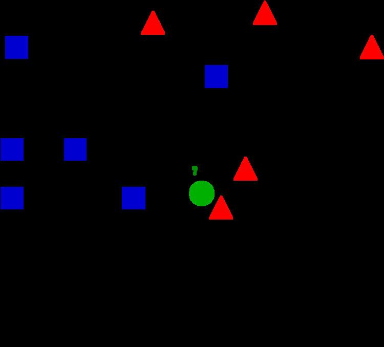
The border ratio is in the interval [0,1] because ||x'-y||never exceeds ||x-y||. This ordering gives preference to the borders of the classes for inclusion in the set of prototypesU. A point of a different label than x is called external to x. The calculation of the border ratio is illustrated by the figure on the right. The data points are labeled by colors: the initial point is x and its label is red. External points are blue and green. The closest to x external point is y. The closest to y red point is x' . The border ratio a(x) = ||x'-y|| / ||x-y||is the attribute of the initial point x.

Below is an illustration of CNN in a series of figures. There are three classes (red, green and blue). Fig. 1: initially there are 60 points in each class. Fig. 2 shows the 1NN classification map: each pixel is classified by 1NN using all the data. Fig. 3 shows the 5NN classification map. White areas correspond to the unclassified regions, where 5NN voting is tied (for example, if there are two green, two red and one blue points among 5 nearest neighbors). Fig. 4 shows the reduced data set. The crosses are the class-outliers selected by the (3,2)NN rule (all the three nearest neighbors of these instances belong to other classes); the squares are the prototypes, and the empty circles are the absorbed points. The left bottom corner shows the numbers of the class-outliers, prototypes and absorbed points for all three classes. The number of prototypes varies from 15% to 20% for different classes in this example. Fig. 5 shows that the 1NN classification map with the prototypes is very similar to that with the initial data set. The figures were produced using the Mirkes applet.

k-NN regression

In k-NN regression, the k-NN algorithm is used for estimating continuous variables. One such algorithm uses a weighted average of the k nearest neighbors, weighted by the inverse of their distance. This algorithm works as follows:

1. Compute the Euclidean or Mahalanobis distance from the query example to the labeled examples.
2. Order the labeled examples by increasing distance.
3. Find a heuristically optimal number k of nearest neighbors, based on RMSE. This is done using cross validation.
4. Calculate an inverse distance weighted average with the k-nearest multivariate neighbors.

k-NN outlier

The distance to the kth nearest neighbor can also be seen as a local density estimate and thus is also a popular outlier score in anomaly detection. The larger the distance to the k-NN, the lower the local density, the more likely the query point is an outlier. Although quite simple, this outlier model, along with another classic data mining method, local outlier factor, works quite well also in comparison to more recent and more complex approaches, according to a large scale experimental analysis.

Validation of results

A confusion matrix or "matching matrix" is often used as a tool to validate the accuracy of k-NN classification. More robust statistical methods such as likelihood-ratio test can also be applied.