Interior reconstruction

Methods

The purpose of each method is to solve for vector x in the following problem:

[ f g ] = [ A B C D ] [ x y ] .

Let X be the region of interest (ROI) and Y be the region outside of X . Assume A , B , C , D are known matrices; x and y are unknown vectors of the original image, while f and g are vector measurements of the responses ( f is known and g is unknown). x is inside region X , ( x ∈ X ) and y , in the region Y , ( y ∈ Y ), is outside region X . f is inside a region in the measurement corresponding to X . This region is denoted as F , ( f ∈ F ), while g is outside of the region F . It corresponds to Y and is denoted as G , ( g ∈ G ).

For CT image-reconstruction purposes, C = 0 .

To simplify the concept of interior reconstruction, the matrices A , B , C , D are applied to image reconstruction instead of complex operators.

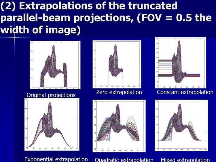
The first interior-reconstruction method listed below is extrapolation. It is a local tomography method which eliminates truncation artifacts but introduces another type of artifact: a bowl effect. An improvement is known as the adaptive extrapolation method, although the iterative extrapolation method below also improves reconstruction results. In some cases, the exact reconstruction can be found for the interior reconstruction. The local inverse method below modifies the local tomography method, and may improve the reconstruction result of the local tomography; the iterative reconstruction method can be applied to interior reconstruction. Among the above methods, extrapolation is often applied.

Extrapolation method

[ f g ] = [ A B C D ] [ x y ]

A , B , C , D are known matrices; x and y are unknown vectors; f is a known vector, and g is an unknown vector. We need to know the vector x . x and y are the original image, while f and g are measurements of responses. Vector x is inside the region of interest X , ( x ∈ X ). Vector y is outside the region X . The outside region is called Y , ( y ∈ Y ) and f is inside a region in the measurement corresponding to X . This region is denoted F , ( f ∈ F ). The region of vector g (outside the region F ) also corresponds to Y and is denoted as G , ( g ∈ G ). In CT image reconstruction, it has

C = 0

To simplify the concept of interior reconstruction, the matrices A , B , C , D are applied to image reconstruction instead of a complex operator.

The response in the outside region can be a guess G ; for example, assume it is g e x

[ x 0 y 0 ] = [ A B C D ] − 1 [ f g e x ]

A solution of x is written as x 0 , and is known as the extrapolation method. The result depends on how good the extrapolation function g e x is. A frequent choice is

g e x | ∂ G = f | ∂ F

at the boundary of the two regions. The extrapolation method is often combined with a priori knowledge, and an extrapolation method which reduces calculation time is shown below.

Adaptive extrapolation method

Assume a rough solution, x 0 and y 0 , is obtained from the extrapolation method described above. The response in the outside region g 1 can be calculated as follows:

g 1 = C x 0 + D y 0

The reconstructed image can be calculated as follows:

[ x 1 y 1 ] = [ A B C D ] − 1 [ f g 1 + g 1 e x ]

It is assumed that

f | ∂ F = ( g 1 + g 1 e x ) | ∂ G

at the boundary of the interior region; x 1 solves the problem, and is known as the adaptive extrapolation method. g 1 e x is the adaptive extrapolation function.

Iterative extrapolation method

It is assumed that a rough solution, x 0 and y 0 , is obtained from the extrapolation method described below:

[ f 1 g 1 ] = [ A B C D ] [ 0 y 0 ]

or

f 1 = B y 0

The reconstruction can be obtained as

[ x 1 y 1 ] = [ A B C D ] − 1 [ f − f 1 g e x ]

Here g 1 e x is an extrapolation function, and it is assumed that

( f − f 1 ) | ∂ F = g 1 e x | ∂ G

x 1 is one solution of this problem.

Local tomography

Local tomography, with a very short filter, is also known as lambda tomography.

Local inverse method

The local inverse method extends the concept of local tomography. The response in the outside region can be calculated as follows:

f = A x + B y

Consider the generalized inverse B + satisfying

B B + B = B

Define

Q = [ I − B B + ]

so that

Q B = 0

Hence,

Q f = Q A x

The above equation can be solved as

x 1 = A + Q + Q f ,

considering that

Q Q = Q Q Q Q = Q

Q is the generalized inverse of Q , i.e.

Q + = Q

The solution can be simplified as

x 1 = A + Q f .

The matrix A + Q = A + [ I − B B + ] is known as the local inverse of matrix [ A B C D ] , corresponding to A . This is known as the local inverse method.

Iterative reconstruction method

Here a goal function is defined, and this method iteratively achieves the goal. If the goal function can be some kind of normal, this is known as the minimal norm method.

min ( R ∥ x ∥ + S ∥ y ∥ + T ∥ g ∥ ) ,

subject to

[ x y ] = [ A B C D ] − 1 [ f g ]

and f is known,

where R , S and T are weighting constants of the minimization and ∥ ⋅ ∥ is some kind of norm. Often-used norms are L 0 , L 1 , L 2 , L + ∞ total variation (TV) norm or a combination of the above norms. An example of this method is the projection onto convex sets (POCS) method.

Analytical solution

In special situations, the interior reconstruction can be obtained as an analytical solution; the solution of x is exact in such cases.

Fast extrapolation

Extrapolated data often convolutes to a kernel function. After data is extrapolated its size is increased N times, where N = 2 ~ 3. If the data needs to be convoluted to a known kernel function, the numerical calculations will increase log(N)·N times, even with the fast Fourier transform (FFT). An algorithm exists, analytically calculating the contribution from part of the extrapolated data. The calculation time can be omitted, compared to the original convolution calculation; with this algorithm, the calculation of a convolution using the extrapolated data is not noticeably increased. This is known as fast extrapolation.

Comparison of methods

The extrapolation method is suitable in a situation where

i.e. a small truncation artifacts situation.

The adaptive extrapolation method is suitable for a situation where

i.e. a normal truncation artifacts situation. This method also offers a rough solution for the exterior region.

The iterative extrapolation method is suitable for a situation in which

i.e. a normal truncation artifacts situation. Although this method gets better interior reconstruction compared to adaptive reconstruction, it misses the result in the exterior region.

Local tomography is suitable for a situation in which

i.e. a largest truncation artifacts situation. Although there are no truncation artifacts in this method, there is a fixed error (independent of the value of | y | ) in the reconstruction.

The local inverse method, identical to local tomography, suitable in a situation in which

i.e. a largest truncation artifacts situation. Although there are no truncation artifacts for this method, there is a fixed error (independent of the value of | y | ) in the reconstruction which may be smaller than with local tomography.

The iterative reconstruction method obtains a good result with large calculations. Although the analytic method achieves an exact result, it is only functional in some situations. The fast extrapolation method can get the same results as the other extrapolation methods, and can be applied to the above interior reconstruction methods to reduce the calculation.