Holonomic constraints - Alchetron, The Free Social Encyclopedia

In classical mechanics, holonomic constraints are relations between the position variables (and possibly time) which can be expressed in the following form: f ( q 1 , q 2 , q 3 , … , q n , t ) = 0 , where { q 1 , q 2 , q 3 , … , q n } are the n coordinates which describe the system. For example, the motion of a particle constrained to lie on the surface of a sphere is subject to a holonomic constraint, but if the particle is able to fall off the sphere under the influence of gravity, the constraint becomes non-holonomic.

Holonomic system (physics)

In classical mechanics a system may be defined as holonomic if all constraints of the system are holonomic. For a constraint to be holonomic it must be expressible as a function:

f ( x 1 , x 2 , x 3 , … , x N , t ) = 0 ,

i.e. a holonomic constraint depends only on the coordinates x j and time t . It does not depend on the velocities or any higher order derivative with respect to t. A constraint that cannot be expressed in the form shown above is a nonholonomic constraint.

Transformation to independent generalized coordinates

The holonomic constraint equations can help us easily remove some of the dependent variables in our system. For example, if we want to remove x d which is a parameter in the constraint equation f i , we can rearrange the equation into the following form, assuming it can be done,

x d = g i ( x 1 , x 2 , x 3 , … , x d − 1 , x d + 1 , … , x N , t ) ,

and replace the x d in every equation of the system using the above function. This can always be done for general physical system, provided that f i is C 1 , then by implicit function theorem, the solution g i is guaranteed in some open set. Thus, it is possible to remove all occurrences of the dependent variable x d .

Suppose that a physical system has N degrees of freedom. Now, h holonomic constraints are imposed on the system. Then, the number of degrees of freedom is reduced to m = N − h . We can use m independent generalized coordinates ( q j ) to completely describe the motion of the system. The transformation equation can be expressed as follows:

x i = x i ( q 1 , q 2 , … , q m , t ) , i = 1 , 2 , … N .

Differential form

Consider the following differential form of a constraint equation:

∑ j c i j d q j + c i d t = 0 ;

where c_ij, c_i are the coefficients of the differentials dq_j and dt for the ith constraint.

If the differential form is integrable, i.e., if there is a function f i ( q 1 , q 2 , q 3 , … , q N , t ) = 0 satisfying the equality

d f i = ∑ j c i j d q j + c i d t = 0 ,

then this constraint is a holonomic constraint; otherwise, nonholonomic. Therefore, all holonomic and some nonholonomic constraints can be expressed using the differential form. Not all nonholonomic constraints can be expressed this way. Examples of nonholonomic constraints which can not be expressed this way are those that are dependent on generalized velocities. With a constraint equation in differential form, whether the constraint is holonomic or nonholonomic depends on the integrability of the differential form.

Classification of physical systems

In order to study classical physics rigorously and methodically, we need to classify systems. Based on previous discussion, we can classify physical systems into holonomic systems and non-holonomic systems. One of the conditions for the applicability of many theorems and equations is that the system must be a holonomic system. For example, if a physical system is a holonomic system and a monogenic system, then Hamilton's principle is the necessary and sufficient condition for the correctness of Lagrange's equation.

Examples

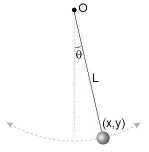
As shown at right, a simple pendulum is a system composed of a weight and a string. The string is attached at the top end to a pivot and at the bottom end to a weight. Being inextensible, the string’s length is a constant. Therefore, this system is holonomic; it obeys the holonomic constraint

x 2 + y 2 − L 2 = 0 ,

where ( x , y ) is the position of the weight and L is length of the string.

The particles of a rigid body obey the holonomic constraint

( r i − r j ) 2 − L i j 2 = 0 ,

where r i , r j are respectively the positions of particles P i and P j , and L i j is the distance between them.

References

Holonomic constraints Wikipedia

(Text) CC BY-SA