Herschel–Bulkley fluid

Definition

The constitutive equation of the Herschel-Bulkley model is commonly written as

τ = τ 0 + k γ ˙ n

where τ is the shear stress, γ ˙ the shear rate, τ 0 the yield stress, k the consistency index, and n the flow index. If τ < τ 0 the Herschel-Bulkley fluid behaves as a solid, otherwise it behaves as a fluid. For n < 1 the fluid is shear-thinning, whereas for n > 1 the fluid is shear-thickening. If n = 1 and τ 0 = 0 , this model reduces to the Newtonian fluid.

As a generalized Newtonian fluid model, the effective viscosity is given as

μ eff = { μ 0 , | γ ˙ | ≤ γ ˙ 0 k | γ ˙ | n − 1 + τ 0 | γ ˙ | − 1 , | γ ˙ | ≥ γ ˙ 0

The limiting viscosity μ 0 is chosen such that μ 0 = k γ ˙ 0 n − 1 + τ 0 γ ˙ 0 − 1 . A large limiting viscosity means that the fluid will only flow in response to a large applied force. This feature captures the Bingham-type behaviour of the fluid.

The viscous stress tensor is given, in the usual way, as a viscosity, multiplied by the rate-of-strain tensor

τ i j = 2 μ eff ( | γ ˙ | ) E i j = μ eff ( | γ ˙ | ) ( ∂ u i ∂ x j + ∂ u j ∂ x i ) ,

where the magnitude of the shear rate is given by

| γ ˙ | = 2 E i j E i j .

The magnitude of the shear rate is an isotropic approximation, and it is coupled with the second invariant of the rate-of-strain tensor

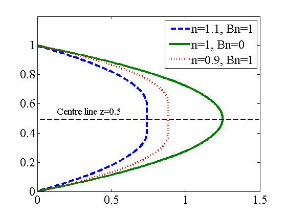
I I E = t r ( E i j E j k ) = E i j E i j .

Channel flow

A frequently-encountered situation in experiments is pressure-driven channel flow (see diagram). This situation exhibits an equilibrium in which there is flow only in the horizontal direction (along the pressure-gradient direction), and the pressure gradient and viscous effects are in balance. Then, the Navier-Stokes equations, together with the rheological model, reduce to a single equation:

∂ p ∂ x = ∂ ∂ z ( μ ∂ u ∂ z ) = { μ 0 ∂ 2 u ∂ z 2 , | ∂ u ∂ z | < γ 0 ∂ ∂ z [ ( k | ∂ u ∂ z | n − 1 + τ 0 | ∂ u ∂ z | − 1 ) ∂ u ∂ z ] , | ∂ u ∂ z | ≥ γ 0

To solve this equation it is necessary to non-dimensionalize the quantities involved. The channel depth H is chosen as a length scale, the mean velocity V is taken as a velocity scale, and the pressure scale is taken to be P 0 = k ( V / H ) n . This analysis introduces the non-dimensional pressure gradient

π 0 = H P 0 ∂ p ∂ x ,

which is negative for flow from left to right, and the Bingham number:

B n = τ 0 k ( H V ) n .

Next, the domain of the solution is broken up into three parts, valid for a negative pressure gradient:

A region close to the bottom wall where ∂ u / ∂ z > γ 0 ;

A region in the fluid core where | ∂ u / ∂ z | < γ 0 ;

A region close to the top wall where ∂ u / ∂ z < − γ 0 ,

Solving this equation gives the velocity profile:

u ( z ) = { n n + 1 1 π 0 [ ( π 0 ( z − z 1 ) + γ 0 n ) 1 + ( 1 / n ) − ( − π 0 z 1 + γ 0 n ) 1 + ( 1 / n ) ] , z ∈ [ 0 , z 1 ] π 0 2 μ 0 ( z 2 − z ) + k , z ∈ [ z 1 , z 2 ] , n n + 1 1 π 0 [ ( − π 0 ( z − z 2 ) + γ 0 n ) 1 + ( 1 / n ) − ( − π 0 ( 1 − z 2 ) + γ 0 n ) 1 + ( 1 / n ) ] , z ∈ [ z 2 , 1 ]

Here k is a matching constant such that u ( z 1 ) is continuous. The profile respects the no-slip conditions at the channel boundaries,

u ( 0 ) = u ( 1 ) = 0 ,

Using the same continuity arguments, it is shown that z 1 , 2 = 1 2 ± δ , where

δ = γ 0 μ 0 | π 0 | ≤ 1 2 .

Since μ 0 = γ 0 n − 1 + B n / γ 0 , for a given ( γ 0 , B n ) pair, there is a critical pressure gradient

| π 0 , c | = 2 ( γ 0 + B n ) .

Apply any pressure gradient smaller in magnitude than this critical value, and the fluid will not flow; its Bingham nature is thus apparent. Any pressure gradient greater in magnitude than this critical value will result in flow. The flow associated with a shear-thickening fluid is retarded relative to that associated with a shear-thinning fluid.

Pipe flow

For laminar flow Chilton and Stainsby provide the following equation to calculate the pressure drop. The equation requires an iterative solution to extract the pressure drop, as it is present on both sides of the equation.

Δ P L = 4 K D ( 8 V D ) n ( 3 n + 1 4 n ) n 1 1 − X ( 1 1 − a X − b X 2 − c X 3 ) n X = 4 L τ y D Δ P a = 1 2 n + 1 b = 2 n ( n + 1 ) ( 2 n + 1 ) c = 2 n 2 ( n + 1 ) ( 2 n + 1 ) For turbulent flow the authors propose a method that requires knowledge of the wall shear stress, but do not provide a method to calculate the wall shear stress. Their procedure is expanded in Hathoot R = 4 n ρ V D ( 1 − a X − b X 2 − c X 3 ) μ W a l l ( 3 n + 1 ) μ W a l l = τ W a l l 1 − 1 / n ( K 1 − X ) 1 / n τ W a l l = D Δ P 4 L All units are SI Δ P Pressure drop, Pa. L Pipe length, m D Pipe diameter, m V Fluid velocity, m / s Chilton and Stainsby state that defining the Reynolds number as R e = R n 2 ( 1 − X ) 4

allows standard Newtonian friction factor correlations to be used.