
 | ||
k trials where k ∈ { 1 , 2 , 3 , … } {\displaystyle k\in \{1,2,3,\dots \}\!} k failures where k ∈ { 0 , 1 , 2 , 3 , … } {\displaystyle k\in \{0,1,2,3,\dots \}\!} ( 1 − p ) k − 1 p {\displaystyle (1-p)^{k-1}\,p\!} ( 1 − p ) k p {\displaystyle (1-p)^{k}\,p\!} 1 − ( 1 − p ) k {\displaystyle 1-(1-p)^{k}\!} 1 − ( 1 − p ) k + 1 {\displaystyle 1-(1-p)^{k+1}\!} 1 p {\displaystyle {\frac {1}{p}}\!} 1 − p p {\displaystyle {\frac {1-p}{p}}\!} ⌈ − 1 log 2 ( 1 − p ) ⌉ {\displaystyle \left\lceil {\frac {-1}{\log _{2}(1-p)}}\right\rceil \!} (not unique if − 1 / log 2 ( 1 − p ) {\displaystyle -1/\log _{2}(1-p)} is an integer) ⌈ − 1 log 2 ( 1 − p ) ⌉ − 1 {\displaystyle \left\lceil {\frac {-1}{\log _{2}(1-p)}}\right\rceil \!-1} (not unique if − 1 / log 2 ( 1 − p ) {\displaystyle -1/\log _{2}(1-p)} is an integer) 1 {\displaystyle 1} 0 {\displaystyle 0} | ||
In probability theory and statistics, the geometric distribution is either of two discrete probability distributions:
Contents
- Introduction to the geometric distribution
- Examples
- Assumptions When is the geometric distribution an appropriate model
- Probability of outcomes
- Expected number of failures before the first success
- Moments and cumulants
- Parameter estimation
- Other properties
- Related distributions
- Geometric distribution using R
- Geometric distribution using Excel
- References
Which of these one calls "the" geometric distribution is a matter of convention and convenience.
These two different geometric distributions should not be confused with each other. Often, the name shifted geometric distribution is adopted for the former one (distribution of the number X); however, to avoid ambiguity, it is considered wise to indicate which is intended, by mentioning the support explicitly.
It’s the probability that the first occurrence of success requires k number of independent trials, each with success probability p. If the probability of success on each trial is p, then the probability that the kth trial (out of k trials) is the first success is
for k = 1, 2, 3, ....
The above form of geometric distribution is used for modeling the number of trials up to and including the first success. By contrast, the following form of the geometric distribution is used for modeling the number of failures until the first success:
for k = 0, 1, 2, 3, ....
In either case, the sequence of probabilities is a geometric sequence.
For example, suppose an ordinary die is thrown repeatedly until the first time a "1" appears. The probability distribution of the number of times it is thrown is supported on the infinite set { 1, 2, 3, ... } and is a geometric distribution with p = 1/6.
Introduction to the geometric distribution
Consider a sequence of trials, where each trial has only two possible outcomes (designated failure and success). The probability of success is assumed to be the same for each trial. In such a sequence of trials, the geometric distribution is useful to model the number of failures before the first success. The distribution gives the probability that there are zero failures before the first success, one failure before the first success, two failures before the first success, and so on.
Examples
A newly-wed couple plans to have children, and will continue until the first girl. What is the probability that there are zero boys before the first girl, one boy before the first girl, two boys before the first girl, and so on?
A doctor is seeking an anti-depressant for a newly diagnosed patient. Suppose that, of the available anti-depressant drugs, the probability that any particular drug will be effective for a particular patient is p=0.6. What is the probability that the first drug found to be effective for this patient is the first drug tried, the second drug tried, and so on? What is the expected number of drugs that will be tried to find one that is effective?
A patient is waiting for a suitable matching kidney donor for a transplant. If the probability that a randomly selected donor is a suitable match is p=0.1, what is the expected number of donors who will be tested before a matching donor is found?
Assumptions: When is the geometric distribution an appropriate model?
The geometric distribution is an appropriate model if the following assumptions are true.
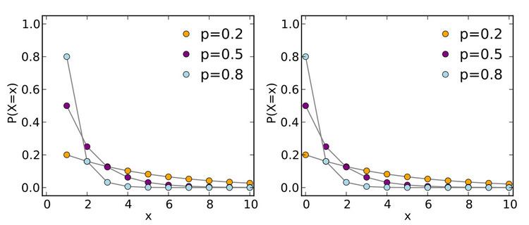
If these conditions are true, then the geometric random variable is the count of the number of failures before the first success. The possible number of failures before the first success is 0, 1, 2, 3, and so on. The geometric random variable Y is the number of failures before the first success. In the graphs above, this formulation is shown on the right.
An alternative formulation is that the geometric random variable X is the total number of trials up to and including the first success, and the number of failures is X-1. In the graphs above, this formulation is shown on the left.
Probability of outcomes
Consider the anti-depressant example above. The probability that any given drug is effective (success) is p=0.6. The probability that a drug will not be effective (fail) is q = 1 – p = 1 – 0.6 = 0.4. Here are probabilities of some possible outcomes.
(i) The first drug works. There are zero failures before the first success. Y = 0 failures. The probability p(zero failures before first success) is simply the probability that the first drug works.
(ii) The first drug fails, but the second drug works. There is one failure before the first success. Y= 1 failure. The probability for this sequence of events is p(first drug fails) \times p(second drug is success) which is given by
(iii) The first drug fails, the second drug fails, but the third drug works. There are two failures before the first success. Y= 2 failures. The probability for this sequence of events is p(first drug fails) \times p(second drug fails) \times p(third drug is success)
The general formula to calculate the probability of k failures before the first success, where the probability of success is p and the probability of failure is q = 1 - p, is
for k = 0, 1, 2, 3, ....
For the newly-weds awaiting their first girl, the probability of no boys before the first girl is
The probability of one boy before the first girl is
The probability of two boys before the first girl is
and so on.
Expected number of failures before the first success
For the geometric distribution, the expected (mean) number of failures before the first success is E(Y) = (1-p)/p.
For the anti-depressant example, with p=0.6, the mean number of failures before the first success is E(Y) = (1-p)/p = (1-0.6)/0.6 = 0.67.
For the kidney-donor example, with p=0.1, the mean number of failures before the first success is E(Y) = (1-0.1)/0.1 = 9.
For the alternative formulation, where X is the number of trials up to and including the first success, the expected value is E(X) = 1/p.
Moments and cumulants
The expected value of a geometrically distributed random variable X is 1/p and the variance is (1 − p)/p2:
Similarly, the expected value of the geometrically distributed random variable Y = X − 1 (where Y corresponds to the pmf listed in the right column) is q/p = (1 − p)/p, and its variance is (1 − p)/p2:
Let μ = (1 − p)/p be the expected value of Y. Then the cumulants
Outline of proof: That the expected value is (1 − p)/p can be shown in the following way. Let Y be as above. Then
(The interchange of summation and differentiation is justified by the fact that convergent power series converge uniformly on compact subsets of the set of points where they converge.)
Parameter estimation
For both variants of the geometric distribution, the parameter p can be estimated by equating the expected value with the sample mean. This is the method of moments, which in this case happens to yield maximum likelihood estimates of p.
Specifically, for the first variant let k = k1, ..., kn be a sample where ki ≥ 1 for i = 1, ..., n. Then p can be estimated as
In Bayesian inference, the Beta distribution is the conjugate prior distribution for the parameter p. If this parameter is given a Beta(α, β) prior, then the posterior distribution is
The posterior mean E[p] approaches the maximum likelihood estimate
In the alternative case, let k1, ..., kn be a sample where ki ≥ 0 for i = 1, ..., n. Then p can be estimated as
The posterior distribution of p given a Beta(α, β) prior is
Again the posterior mean E[p] approaches the maximum likelihood estimate
Other properties
Related distributions
Since:
Geometric distribution using R
The R function dgeom(k, prob) calculates the probability that there are k failures before the first success, where the argument "prob" is the probability of success on each trial.
For example,
dgeom(0,0.6) = 0.6
dgeom(1,0.6) = 0.24
R uses the convention that k is the number of failures, so that the number of trials up to and including the first success is k + 1.
The following R code creates a graph of the geometric distribution from Y= 0 to 10, with p=0.6.
Y=0:10
plot(Y, dgeom(Y,0.6), type="h", ylim=c(0,1), main="Geometric distribution for p=0.6", ylab="P(Y=Y)", xlab="Y=Number of failures before first success")
Geometric distribution using Excel
The geometric distribution, for the number of failures before the first success, is a special case of the negative binomial distribution, for the number of failures before s successes.
The Excel function NEGBINOMDIST(number_f, number_s, probability_s) calculates the probability of k = number_f failures before s = number_s successes where p = probability_s is the probability of success on each trial. For the geometric distribution, let number_s = 1 success.
For example,
=NEGBINOMDIST(0, 1, 0.6) = 0.6
=NEGBINOMDIST(1, 1, 0.6) = 0.24
Like R, Excel uses the convention that k is the number of failures, so that the number of trials up to and including the first success is k + 1.