
 | ||
In mathematics, a generalized conic is a geometrical object defined by a property which is a generalization of some defining property of the classical conic. For example, in elementary geometry, an ellipse can be defined as the locus of a point which moves in a plane such that the sum of its distances from two fixed points in the plane is a constant. The curve obtained when the set of two fixed points is replaced by an arbitrary, but fixed, finite set of points in the plane can be thought of as a generalized ellipse. Since an ellipse is the equidistant set of two circles, the equidistant set of two arbitrary sets of points in a plane can be viewed as a generalized conic. In rectangular Cartesian coordinates, the equation y = x2 represents a parabola. The generalized equation y = xr, for r ≠ 0 and r ≠ 1, can be treated as defining a generalized parabola. The idea of generalized conic has found applications in approximation theory and optimization theory.
Contents
- Multifocal oval curves
- Definition
- Specialization and generalization of Maxwells approach
- Generalized conics via polar equations
- Special cases
- Generalized conics in curve approximation
- Examples
- References
Among the several possible ways in which the concept of a conic can be generalized, the most widely used approach is to define it as a generalization of the ellipse. The starting point for this approach is to look upon an ellipse as a curve satisfying the 'two-focus property': an ellipse is a curve that is the locus of points the sum of whose distances from two given points is constant. The two points are the foci of the ellipse. The curve obtained by replacing the set of two fixed points by an arbitrary, but fixed, finite set of points in the plane can be thought of as a generalized ellipse. Generalized conics with three foci are called trifocal ellipses. This can be further generalized to curves which are obtained as the loci of points which move such that the some of weighted arithmetic mean of the distances from a finite set of points is a constant. A still further generalization is possible by assuming that the weights attached to the distances can be of arbitrary sign, namely, plus or minus. Finally, the restriction that the set of fixed points, called the set of foci of the generalized conic, be finite may also be removed. The set may be assumed to be finite or infinite. In the infinite case, the weighted arithmetic mean has to be replaced by an appropriate integral. Generalized conics in this sense are also called polyellipses, egglipses, or, generalized ellipses. Since such curves were considered by the German mathematician Ehrenfried Walther von Tschirnhaus (1651 – 1708) they are also known as Tschirnhaus'sche Eikurve. Also such generalizations have been discussed by Rene Descartes and by James Clerk Maxwell.
Multifocal oval curves
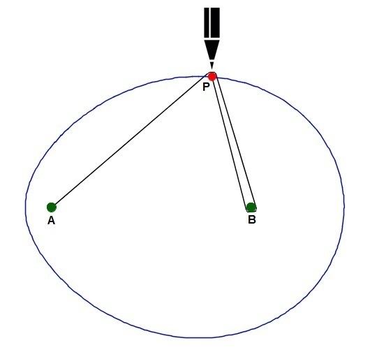
Rene Descartes (1596–1650), father of analytical geometry, in his La Geometrie published in 1637, set apart a section of about 15 pages to discuss what he had called bifocal ellipses. A bifocal oval was defined there as the locus of a point P which moves in a plane such that
Multifocal ovals were rediscovered by James Clerk Maxwell (1831–1879) while he was still a school student. At the young age of 15, Maxwell wrote a scientific paper on these ovals with the title "Observations on circumscribed figures having a plurality of foci, and radii of various proportions" and got it presented by Professor J. D. Forbes in a meeting of the Royal Society of Edinburgh in 1846. Professor J. D. Forbes also published an account of the paper in the Proceedings of Royal Society of Edinburgh. In his paper, though Maxwell did not use the term "generalized conic", he was considering curves defined by conditions which were generalizations of the defining condition of an ellipse.
Definition
A multifocal oval is a curve which is defined as the locus of a point moving such that
where A1, A2, . . . , An are fixed points in a plane and λ1, λ2, . . . , λn are fixed rational numbers and c is a constant. He gave simple pin-string-pencil methods for drawing such ovals.
The method for drawing the oval defined by the equation
In the next two years since his paper was presented in the Royal Society of Edinburgh, Maxwell systematically developed the geometrical and optical properties of these ovals.
Specialization and generalization of Maxwell's approach
As a special case of Maxwell's approach, consider the locus of a point which moves such that the following condition is satisfied:
Dividing by n and replacing c/n by c, this defining condition can be stated as
This suggests a simple interpretation: the generalised conic is a curve such that the average distance of every point P on the curve from the set {A1, A2, . . . , An} has the same constant value. This formulation of the concept of a generalized conic has been further generalised in several different ways.
The formulation of the definition of the generalized conic in the most general case when the cardinality of the focal set is infinite involves the notions of measurable sets and Lebesgue integration. All these have been employed by different authors and the resulting curves have been studied with special emphasis on applications.
Definition
Let
where
Generalized conics via polar equations
Given a conic, by choosing a focus of the conic as the pole and the line through the pole drawn parallel to the directrix of the conic as the polar axis, the polar equation of the conic can be written in the following form:
Here e is the eccentricity of the conic and d is the distance of the directrix from the pole. Tom M. Apostol and Mamikon A. Mnatsakanian in their study of curves drawn on the surfaces of right circular cones introduced a new class of curves which they called generalized conics. These are curves whose polar equations are similar to the polar equations of ordinary conics and the ordinary conics appear as special cases of these generalized conics.
Definition
For constants r0 ≥ 0, λ ≥ 0 and real k, a plane curve described by the polar equation
is called a generalized conic. The conic is called a generalized ellipse, parabola or hyperbola according as λ < 1, λ = 1, or λ > 1.
Special cases
Generalized conics in curve approximation
In 1996, Ruibin Qu introduced a new notion of generalized conic as a tool for generating approximations to curves. The starting point for this generalization is the result that the sequence of points
lie on a conic. In this approach, the generalized conic is now defined as below.
Definition
A generalized conic is such a curve that if the two points
for some
are also on it.
Definition
Let (X, d) be a metric space and let A be a nonempty subset of X. If x is a point in X, the distance of x from A is defined as d(x, A) = inf{ d(x, a): a in A}. If A and B are both nonempty subsets of X then the equidistant set determined by A and B is defined to be the set {x in X: d(x, A) = d(x, B)}. This equidistant set is denoted by { A = B }. The term generalized conic is used to denote a general equidistant set.
Examples
Classical conics can be realized as equidistant sets. For example, if A is a singleton set and B is a straight line, then the equidistant set { A = B } is a parabola. If A and B are circles such that A is completely within B then the equidistant set { A = B } is an ellipse. On the other hand, if A lies completely outside B the equidistant set { A = B } is a hyperbola.