Gaussian network model

Gaussian network model theory

The Gaussian network model was proposed by Bahar, Atilgan, Haliloglu and Erman in 1997, motivated by a study by Tirion, I. Tirion showed by normal mode analysis that the representation of atomic interactions by harmonic potentials with uniform spring constant (instead of detailed force field functions and parameters) would not alter the most collective modes of motions predicted at the lowest frequency end of the spectrum, in accord with earlier works that utilized normal mode analysis and simplified harmonic potentials to study the dynamics. The GNM differs from normal mode analyses and simulations, as it offers an analytical formulation and unique solution for each structure, exclusively based on inter-residue contact topology, influenced by the theory of elasticity of Flory and the Rouse model

Representation of structure as an elastic network

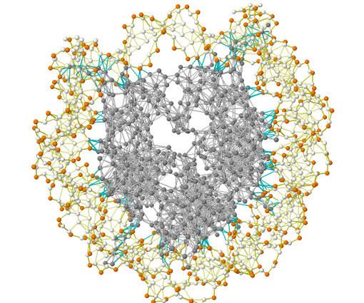
Figure 2 shows a schematic view of elastic network studied in GNM. Metal beads represent the nodes in this Gaussian network (residues of a protein) and springs represent the connections between the nodes (covalent and non-covalent interactions between residues). For nodes i and j, equilibrium position vectors, R⁰_i and R⁰_j, equilibrium distance vector, R⁰_ij, instantaneous fluctuation vectors, ΔR_i and ΔR_j, and instantaneous distance vector, R_ij, are shown in Figure 2. Instantaneous position vectors of these nodes are defined by R_i and R_j. The difference between equilibrium position vector and instantaneous position vector of residue i gives the instantaneous fluctuation vector, ΔR_i = R_i - R⁰_i. Hence, the instantaneous fluctuation vector between nodes i and j is expressed as ΔR_ij = ΔR_j - ΔR_i = R_ij - R⁰_ij.

Potential of the Gaussian network

The potential energy of the network in terms of ΔR_i is

V G N M = γ 2 [ ∑ i , j N ( Δ R j − Δ R i ) 2 ] = γ 2 [ ∑ i , j N Δ R i Γ i j Δ R j ]

where γ is a force constant uniform for all springs and Γ_ij is the ijth element of the Kirchhoff (or connectivity) matrix of inter-residue contacts, Γ, defined by

Γ i j = { − 1 , if  i ≠ j and  R i j ≤ r c 0 , if  i ≠ j and  R i j > r c − ∑ j , j ≠ i N Γ i j , if  i = j

r_c is a cutoff distance for spatial interactions and taken to be 7 Å for amino acid pairs (represented by their α-carbons).

Expressing the X, Y and Z components of the fluctuation vectors ΔR_i as ΔX^T = [ΔX₁ ΔX₂ ..... ΔX_N], ΔY^T = [ΔY₁ ΔY₂ ..... ΔY_N], and ΔZ^T = [ΔZ₁ ΔZ₂ ..... ΔZ_N], above equation simplifies to

V G N M = γ 2 [ Δ X T Γ Δ X + Δ Y T Γ Δ Y + Δ Z T Γ Δ Z ]

Statistical mechanics foundations

In the GNM, the probability distribution of all fluctuations, P(ΔR) is isotropic

P ( Δ R ) = P ( Δ X , Δ Y , Δ Z ) = p ( Δ X ) p ( Δ Y ) p ( Δ Z )

and Gaussian

p ( Δ X ) ∝ exp ⁡ { − γ 2 k B T Δ X T Γ Δ X } = exp ⁡ { − 1 2 ( Δ X T ( k B T γ Γ − 1 ) − 1 Δ X ) }

where k_B is the Boltzmann constant and T is the absolute temperature. p(ΔY) and p(ΔZ) are expressed similarly. N-dimensional Gaussian probability density function with random variable vector x, mean vector μ and covariance matrix Σ is

W ( x , μ , Σ ) = 1 ( 2 π ) N | Σ | exp ⁡ { − 1 2 ( x − μ ) T Σ − 1 ( x − μ ) }

( 2 π ) N | Σ | normalizes the distribution and |Σ| is the determinant of the covariance matrix.

Similar to Gaussian distribution, normalized distribution for ΔX^T = [ΔX₁ ΔX₂ ..... ΔX_N] around the equilibrium positions can be expressed as

p ( Δ X ) = 1 ( 2 π ) N k B T γ | Γ − 1 | exp ⁡ { − 1 2 ( Δ X T ( k B T γ Γ − 1 ) − 1 Δ X ) }

The normalization constant, also the partition function Z_X, is given by

Z X = ∫ 0 ∞ exp ⁡ { − 1 2 ( Δ X T ( k B T γ Γ − 1 ) − 1 Δ X ) } d Δ X

where k B T γ Γ − 1 is the covariance matrix in this case. Z_Y and Z_Z are expressed similarly. This formulation requires inversion of the Kirchhoff matrix. In the GNM, the determinant of the Kirchhoff matrix is zero, hence calculation of its inverse requires eigenvalue decomposition. Γ⁻¹ is constructed using the N-1 non-zero eigenvalues and associated eigenvectors. Expressions for p(ΔY) and p(ΔZ) are similar to that of p(ΔX). The probability distribution of all fluctuations in GNM becomes

P ( Δ R ) = p ( Δ X ) p ( Δ Y ) p ( Δ Z ) = 1 ( 2 π ) 3 N | k B T γ Γ − 1 | 3 exp ⁡ { − 3 2 ( Δ X T ( k B T γ Γ − 1 ) − 1 Δ X ) }

For this mass and spring system, the normalization constant in the preceding expression is the overall GNM partition function, Z_GNM,

Z G N M = Z X Z Y Z Z = 1 ( 2 π ) 3 N | k B T γ Γ − 1 | 3

Expectation values of fluctuations and correlations

The expectation values of residue fluctuations, <ΔR_i²> (also called mean-square fluctuations, MSFs), and their cross-correlations, <ΔR_i · ΔR_j> can be organized as the diagonal and off-diagonal terms, respectively, of a covariance matrix. Based on statistical mechanics, the covariance matrix for ΔX is given by

< Δ X ⋅ Δ X T >= ∫ Δ X ⋅ Δ X T p ( Δ X ) d Δ X = k B T γ Γ − 1

The last equality is obtained by inserting the above p(ΔX) and taking the (generalized Gaussian) integral. Since,

< Δ X ⋅ Δ X T >=< Δ Y ⋅ Δ Y T >=< Δ Z ⋅ Δ Z T >= 1 3 < Δ R ⋅ Δ R T >

<ΔR_i²> and <ΔR_i · ΔR_j> follows

< Δ R i 2 >= 3 k B T γ ( Γ − 1 ) i i < Δ R i ⋅ Δ R j >= 3 k B T γ ( Γ − 1 ) i j

Mode decomposition

The GNM normal modes are found by diagonalization of the Kirchhoff matrix, Γ = UΛU^T. Here, U is a unitary matrix, U^T = U⁻¹, of the eigenvectors u_i of Γ and Λ is the diagonal matrix of eigenvalues λ_i. The frequency and shape of a mode is represented by its eigenvalue and eigenvector, respectively. Since the Kirchhoff matrix is positive semi-definite, the first eigenvalue, λ₁, is zero and the corresponding eigenvector have all its elements equal to 1/√N. This shows that the network model translationally invariant.

Cross-correlations between residue fluctuations can be written as a sum over the N-1 nonzero modes as

< Δ R i ⋅ Δ R j >= 3 k B T γ [ U Λ − 1 U T ] i j = 3 k B T γ ∑ k = 1 N − 1 λ k − 1 [ u k u k T ] i j

It follows that, [ΔR_i · ΔR_j], the contribution of an individual mode is expressed as

[ Δ R i ⋅ Δ R j ] k = 3 k B T γ λ k − 1 [ u k ] i [ u k ] j

where [u_k]_i is the ith element of u_k.

Influence of local packing density

By definition, a diagonal element of the Kirchhoff matrix, Γ_ii, is equal to the degree of a node in GNM that represents the corresponding residue’s coordination number. This number is a measure of the local packing density around a given residue. The influence of local packing density can be assessed by series expansion of Γ⁻¹ matrix. Γ can be written as a sum of two matrices, Γ = D + O, containing diagonal elements and off-diagonal elements of Γ.

Γ⁻¹ = (D + O)⁻¹ = [ D (I + D⁻¹O) ]⁻¹ = (I + D⁻¹O)⁻¹D⁻¹ = (I - D⁻¹O + ...)⁻¹D⁻¹ = D⁻¹ - D⁻¹O D⁻¹ + ...

This expression shows that local packing density makes a significant contribution to expected fluctuations of residues. The terms that follow inverse of the diagonal matrix, are contributions of positional correlations to expected fluctuations.

Equilibrium fluctuations

Equilibrium fluctuations of biological molecules can be experimentally measured. In X-ray crystallography the B-factor (also called Debye-Waller or temperature factor) of each atom is a measure of its mean-square fluctuation near its equilibrium position in the native structure. In NMR experiments, this measure can be obtained by calculating root-mean-square differences between different models. In many applications and publications, including the original articles, it has been shown that has been shown that expected residue fluctuations obtained by the GNM are in good agreement with the experimentally measured native state fluctuations. The relation between B-factors, for example, and expected residue fluctuations obtained from GNM is as follows

B i = 8 π 2 3 < Δ R i ⋅ Δ R i >= 8 π 2 k B T γ ( Γ − 1 ) i i

Figure 3 shows an example of GNM calculation for the catalytic domain of the protein Cdc25B, a cell division cycle dual-specificity phosphatase.

Physical meanings of slow and fast modes

Diagonalization of the Kirchhoff matrix decomposes the conformational motions into a spectrum of collective modes. The expected values of fluctuations and cross-correlations are obtained from linear combinations of fluctuations along these normal modes. The contribution of each mode is scaled with the inverse of that modes frequency. Hence, slow (low frequency) modes contribute most to the expected fluctuations. Along the few slowest modes, motions are shown to be collective and global and potentially relevant to functionality of the biomolecules [9,13,15-18]. Fast (high frequency) modes, on the other hand, describe uncorrelated motions not inducing notable changes in the structure.

Other specific applications

There are several major areas in which the Gaussian network model and other elastic network models have proved to be useful. These include:

Spring bead based network model: In spring-bead based network model, the springs and beads are used as components in the crosslinked network. Springs are cross-linked to represent mechanical behavior of the material and bridge molecular dynamics (MD) model and finite element (FE) model (see Figure. 5). The beads represent material mass of cluster bonds. Each spring is used to represent a cluster of polymer chains, instead of part of a single polymer chain. This simplification allows to bridge different models at multiple length scales and improves the simulation efficiency significantly. At each iteration step in the simulation, forces in the springs are applied to the nodes at the center of the beads, and the equilibrated nodal displacements throughout the system are calculated. Different from the traditional FE method for obtaining stress and strain, the spring–bead model provides the displacements of the nodes and forces in the springs. The equivalent strain and strain energy of spring–bead based network model can be defined and calculated using the displacements of nodes and the spring characteristics. Furthermore, the results from the network model can be scaled up to obtain the structural response at the macroscale using FE analysis.

Decomposition of flexible/rigid regions and domains of proteins

Characterization of functional motions and functionally important sites/residues of proteins, enzymes and large macromolecular assemblies

Refinement and dynamics of low-resolution structural data, e.g. Cryo-electron microscopy

Molecular replacement for solving X-ray structures, when a conformational change occurred, with respect to a known structure

Integration with atomistic models and simulations

Investigation of folding/unfolding pathways and kinetics.

Annotation of functional implication in molecular evolution

Web servers

In practice, two kinds of calculations can be performed. The first kind (the GNM per se) makes use of the Kirchhoff matrix. The second kind (more specifically called either the Elastic Network Model or the Anisotropic Network Model) makes use of the Hessian matrix associated to the corresponding set of harmonic springs. Both kinds of models can be used online, using the following servers.

GNM servers

iGNM: A database of protein functional motions based on GNM http://ignm.ccbb.pitt.edu

oGNM: Online calculation of structural dynamics using GNM http://web.archive.org/web/20070516042756/http://ignm.ccbb.pitt.edu:80/GNM_Online_Calculation.htm

ENM/ANM servers

Anisotropic Network Model web server http://www.ccbb.pitt.edu/anm

elNemo: Web-interface to The Elastic Network Model http://www.sciences.univ-nantes.fr/elnemo/

AD-ENM: Analysis of Dynamics of an Elastic Network Model http://enm.lobos.nih.gov/

WEBnm@: Web-server for Normal Mode Analysis of proteins http://apps.cbu.uib.no/webnma/home

Other relevant servers

ProDy: An Application Programming Interface (API) in Python, that integrates GNM and ANM analyses and several molecular structure and sequence analyses and visualization tools: http://prody.csb.pitt.edu

HingeProt: An algorithm for protein hinge prediction using elastic network models http://www.prc.boun.edu.tr/appserv/prc/hingeprot/, or http://bioinfo3d.cs.tau.ac.il/HingeProt/hingeprot.html

DNABindProt: A Server for Determination of Potential DNA Binding Sites of Proteins http://www.prc.boun.edu.tr/appserv/prc/dnabindprot/

MolMovDB: A database of macromolecular motions: http://www.molmovdb.org/