Anisotropic Network Model

Theory

The Anisotropic Network Model was introduced in 2000 (Atilgan et al., 2001; Doruker et al., 2000), inspired by the pioneering work of Tirion (1996), succeeded by the development of the Gaussian network model (GNM) (Bahar et al., 1997; Haliloglu et al., 1997), and by the work of Hinsen (1998) who first demonstrated the validity of performing EN NMA at residue level.
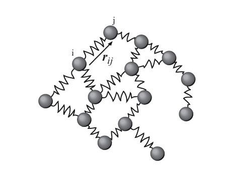
It represents the biological macromolecule as an elastic mass-and-spring network, to explain the internal motions of a protein subject to a harmonic potential. In the network each node is the Cα atom of the residue and the springs represent the interactions between the nodes. The overall potential is the sum of harmonic potentials between interacting nodes. To describe the internal motions of the spring connecting the two atoms, there is only one degree of freedom. Qualitatively, this corresponds to the compression and expansion of the spring in a direction given by the locations of the two atoms. In other words, ANM is an extension of the Gaussian Network Model to three coordinates per atom, thus accounting for directionality.

The network includes all interactions within a cutoff distance, which is the only predetermined parameter in the model. Information about the orientation of each interaction with respect to the global coordinates system is considered within the Force constant matrix (H) and allows prediction of anisotropic motions. Consider a sub-system consisting of nodes i and j, let r_i = (x_i y_i z_i) and let r_j = (x_j y_j z_j) be the instantaneous positions of atoms i and j. The equilibrium distance between the atoms is represented by s_ij^O and the instantaneous distance is given by s_ij. For the spring between i and j, the harmonic potential in terms of the unknown spring constant γ, is given by:

V i j = γ 2 ( s i j − s i j o ) 2

The second derivatives of the potential, V_ij with respect to the components of r_i are evaluated at the equilibrium position, i.e. s_ij^O = s_ij, are

∂ 2 V i j ∂ x i 2 = ∂ 2 V i j ∂ x j 2 = γ s i j 2 ( x j − x i ) 2

∂ 2 V i j ∂ x i ∂ y j = − γ s i j 2 ( x j − x i ) ( y j − y i )

The force constant of the system can be described by the Hessian Matrix – (second partial derivative of potential V):

H = [ H i i H i j H j i H j j ]

Each element Hi,j is a 3×3 matrix which holds the anisotropic information regarding the orientation of nodes i,j. Each such sub matrix (or the "super element" of the Hessian) is defined as:

H i j = [ ∂ 2 V i j ∂ x i ∂ x j ∂ 2 V i j ∂ x i ∂ y j ∂ 2 V i j ∂ x i ∂ z j ∂ 2 V i j ∂ y i ∂ x j ∂ 2 V i j ∂ y i ∂ y j ∂ 2 V i j ∂ y i ∂ z j ∂ 2 V i j ∂ z i ∂ x j ∂ 2 V i j ∂ z i ∂ y j ∂ 2 V i j ∂ z i ∂ z j ]

Using the definition of the potential, the Hessian can be expanded as,

H i j = − γ s i j 2 [ ( x j − x i ) ( x j − x i ) ( x j − x i ) ( y j − y i ) ( x j − x i ) ( z j − z i ) ( y j − y i ) ( x j − x i ) ( y j − y i ) ( y j − y i ) ( y j − y i ) ( z j − z i ) ( z j − z i ) ( x j − x i ) ( z j − z i ) ( y j − y i ) ( z j − z i ) ( z j − z i ) ]

which can then be written as,

H i j = − γ s i j 2 [ x j − x i y j − y i z j − z i ] [ x j − x i y j − y i z j − z i ]

Here, the force constant matrix, or the hessian matrix H holds information about the orientation of the nodes, but not about the type of the interaction (such is whether the interaction is covalent or non-covalent, hydrophobic or non-hydrophobic, etc.). In addition, the distance between the interacting nodes is not considered directly. To account for the distance between the interactions we can weight each interaction between nodes i, j by the distance, sp. The new off-diagonal elements of the Hessian matrix take the below form, where p is an empirical parameter:
H i j = − 1 s i j p + 2 [ ( X j − X i ) ( X j − X i ) ( X j − X i ) ( Y j − Y i ) ( X j − X i ) ( Z j − Z i ) ( Y j − Y i ) ( X j − X i ) ( Y j − Y i ) ( Y j − Y i ) ( Y j − Y i ) ( Z j − Z i ) ( Z j − Z i ) ( X j − X i ) ( Z j − Z i ) ( Y j − Y i ) ( Z j − Z i ) ( Z j − Z i ) ]

The counterpart of the Kirchhoff matrix Γ of the GNM is simply (1/γ) Η in the ANM. Its decomposition yields 3N - 6 non-zero eigenvalues, and 3N - 6 eigenvectors that reflect the respective frequencies and shapes of the individual modes. The inverse of Η, which holds the desired information about fluctuations is composed of N x N super-elements, each of which scales with the 3 x 3 matrix of correlations between the components of pairs of fluctuation vectors. The Hessian, however is not invertible, as its rank is 3N-6 (6 variables responsible to a rigid body motion). To obtain a pseudo inverse, a solution to the eigenvalue problem is obtained:

H = U Λ U T

The pseudo-inverse is composed of the 3N-6 eigenvectors and their respective non-zero eigen values. Where λi are the eigenvalues of H sorted by their size from small to large and Ui the corresponding eigenvectors. The eigenvectors (the columns of the matrix U) describe the vibrational direction and the relative amplitude in the different modes.

Comparing ANM and GNM

ANM and GNM are both based on an elastic network model. The GNM has proven itself to accurately describe the vibrational dynamics of proteins and their complexes in numerous studies. Whereas the GNM is limited to the evaluation of the mean squared displacements and cross-correlations between fluctuations, the motion being projected to a mode space of N dimensions, the ANM approach permits us to evaluate directional preferences and thus provides 3-D descriptions of the 3N - 6 internal modes.

It has been observed that GNM fluctuation predictions agree better with experiments than those computed with ANM. The higher performance of GNM can been attributed to its underlying potential, which takes account of orientational deformations, in addition to distance changes.

Evaluation of the Model

ANM has been evaluated on a large set of proteins to establish the optimal model parameters that achieve the highest correlation with experimental data and its limits of accuracy and applicability. The ANM is evaluated by comparing the fluctuations predicted from theory and those experimentally observed (B-factors deposited in the PDB). During evaluation, the following observations have been made about the models behavior.

Applications of ANM

Recent notable applications of ANM where it has proved to be a promising tool for describing the collective dynamics of the bio-molecular system, include the studies of:
- Hemoglobin, by Chunyan et al., 2003.
- Influenza virus Hemagglutinin A, by Isin et al., 2002.
- Tubulin, by Keskin et al., 2002.
- HIV-1 reverse transcriptase complexed with different inhibitors, by Temiz and Bahar, 2002.
- HIV-1 protease, by Micheletti et al., 2004; Vincenzo et al., 2006.
- DNA-polymerase, by Delarue and Sanejouand, 2002.
- Motor proteins, by Zheng and Brooks, 2005; Zheng and Brooks, 2005; Zheng and Doniach, 2003.
- Membrane proteins including potassium channels, by Shrivastava and Bahar, 2006.
- Rhodopsin, by Rader et al., 2004.
- Nicotinic acetylcholine receptor, by Hung et al., 2005; Taly et al., 2005 and a few more.

ANM Web Servers

The ANM web server developed by Eyal E, Yang LW, Bahar I. in 2006, presents a web-based interface for performing ANM calculations, the main strengths of which are the rapid computing ability and the user-friendly graphical capabilities for analyzing and interpreting the outputs.
- Anisotropic Network Model web server. [1]
- ANM server. [2]