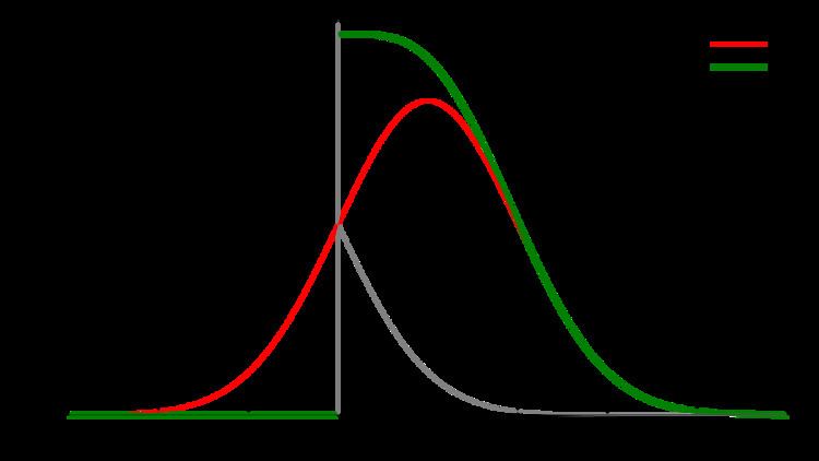
Support x ∈ [0,∞) | ||
 | ||
Parameters μ ∈ R (location)
σ > 0 (scale) PDF 1
σ
2
π
e
−
(
x
−
μ
)
2
2
σ
2
+
1
σ
2
π
e
−
(
x
+
μ
)
2
2
σ
2
{\displaystyle {\frac {1}{\sigma {\sqrt {2\pi }}}}\,e^{-{\frac {(x-\mu )^{2}}{2\sigma ^{2}}}}+{\frac {1}{\sigma {\sqrt {2\pi }}}}\,e^{-{\frac {(x+\mu )^{2}}{2\sigma ^{2}}}}} CDF 1
2
[
erf
(
x
+
μ
σ
2
)
+
erf
(
x
−
μ
σ
2
)
]
{\displaystyle {\frac {1}{2}}\left[{\mbox{erf}}\left({\frac {x+\mu }{\sigma {\sqrt {2}}}}\right)+{\mbox{erf}}\left({\frac {x-\mu }{\sigma {\sqrt {2}}}}\right)\right]} Mean μ
Y
=
σ
2
π
e
(
−
μ
2
/
2
σ
2
)
+
μ
(
1
−
2
Φ
(
−
μ
σ
)
)
{\displaystyle \mu _{Y}=\sigma {\sqrt {\tfrac {2}{\pi }}}\,e^{(-\mu ^{2}/2\sigma ^{2})}+\mu \left(1-2\,\Phi ({\tfrac {-\mu }{\sigma }})\right)} Variance σ
Y
2
=
μ
2
+
σ
2
−
μ
Y
2
{\displaystyle \sigma _{Y}^{2}=\mu ^{2}+\sigma ^{2}-\mu _{Y}^{2}} | ||
The folded normal distribution is a probability distribution related to the normal distribution. Given a normally distributed random variable X with mean μ and variance σ2, the random variable Y = |X| has a folded normal distribution. Such a case may be encountered if only the magnitude of some variable is recorded, but not its sign. The distribution is called Folded because probability mass to the left of the x = 0 is "folded" over by taking the absolute value. In the physics of heat conduction, the folded normal distribution is a fundamental solution of the heat equation on the upper plane (i.e. a heat kernel).
Contents
- Mode of the distribution
- Characteristic function and other related functions
- Parameter estimation
- Differential equations
- Related distributions
- References
The probability density function (PDF) is given by
for x≥0, and 0 everywhere else. An alternative formulation is given by
where cosh is the cosine Hyperbolic function. It follows that the cumulative distribution function (CDF) is given by:
for x≥0, where erf() is the error function. This expression reduces to the CDF of the half-normal distribution when μ = 0.
The mean of the folded distribution is then
or
where
The variance then is expressed easily in terms of the mean:
Both the mean (μ) and variance (σ2) of X in the original normal distribution can be interpreted as the location and scale parameters of Y in the folded distribution.
Mode of the distribution
The mode of the distribution is the value of
Tsagris et al. (2014) saw from numerical investigation that when
Characteristic function and other related functions
Parameter estimation
There are a few ways of estimating the parameters of the folded normal are presented. All of them are essentially the maximum likelihood estimation procedure, but in the some cases, a numerical maximization is performed, whereas in other cases, the root of an equation is being searched. The log-likelihood of the folded normal when a sample
In R (programming language) the command optim or nlm will do the job. The maximisation is fast and easy, since two parameters (
The partial derivatives of the log-likelihood are written as
By equating the first partial derivative of the log-likelihood to zero, we obtain a nice relationship
Note that the above equation has three solutions, one at zero and two more with the opposite sign. By substituting the above equation, to the partial derivative of the log-likelihood w.r.t
which is the same formula as in the normal distribution. A main difference here is that
It becomes clear that the optimization the log-likelihood with respect to the two parameters has turned into a root search of a function. This of course is identical to the previous root search. Tsagris et al. (2014) spotted that there are three roots to this equation for
Differential equations
The PDF of the folded normal distribution can also be defined by the system of differential equations
