Fluorescence correlation spectroscopy - Alchetron, the free social encyclopedia

Fluorescence correlation spectroscopy (FCS) is a correlation analysis of fluctuation of the fluorescence intensity. The analysis provides parameters of the physics under the fluctuations. One of the interesting applications of this is an analysis of the concentration fluctuations of fluorescent particles (molecules) in solution. In this application, the fluorescence emitted from a very tiny space in solution containing a small number of fluorescent particles (molecules) is observed. The fluorescence intensity is fluctuating due to Brownian motion of the particles. In other words, the number of the particles in the sub-space defined by the optical system is randomly changing around the average number. The analysis gives the average number of fluorescent particles and average diffusion time, when the particle is passing through the space. Eventually, both the concentration and size of the particle (molecule) are determined. Both parameters are important in biochemical research, biophysics, and chemistry.

FCS is such a sensitive analytical tool because it observes a small number of molecules (nanomolar to picomolar concentrations) in a small volume (~1μm³). In contrast to other methods (such as HPLC analysis) FCS has no physical separation process; instead, it achieves its spatial resolution through its optics. Furthermore, FCS enables observation of fluorescence-tagged molecules in the biochemical pathway in intact living cells. This opens a new area, "in situ or in vivo biochemistry": tracing the biochemical pathway in intact cells and organs.

Commonly, FCS is employed in the context of optical microscopy, in particular Confocal microscopy or two-photon excitation microscopy. In these techniques light is focused on a sample and the measured fluorescence intensity fluctuations (due to diffusion, physical or chemical reactions, aggregation, etc.) are analyzed using the temporal autocorrelation. Because the measured property is essentially related to the magnitude and/or the amount of fluctuations, there is an optimum measurement regime at the level when individual species enter or exit the observation volume (or turn on and off in the volume). When too many entities are measured at the same time the overall fluctuations are small in comparison to the total signal and may not be resolvable – in the other direction, if the individual fluctuation-events are too sparse in time, one measurement may take prohibitively too long. FCS is in a way the fluorescent counterpart to dynamic light scattering, which uses coherent light scattering, instead of (incoherent) fluorescence.

When an appropriate model is known, FCS can be used to obtain quantitative information such as

diffusion coefficients

hydrodynamic radii

average concentrations

kinetic chemical reaction rates

singlet-triplet dynamics

Because fluorescent markers come in a variety of colors and can be specifically bound to a particular molecule (e.g. proteins, polymers, metal-complexes, etc.), it is possible to study the behavior of individual molecules (in rapid succession in composite solutions). With the development of sensitive detectors such as avalanche photodiodes the detection of the fluorescence signal coming from individual molecules in highly dilute samples has become practical. With this emerged the possibility to conduct FCS experiments in a wide variety of specimens, ranging from materials science to biology. The advent of engineered cells with genetically tagged proteins (like green fluorescent protein) has made FCS a common tool for studying molecular dynamics in living cells.

History

Signal-correlation techniques were first experimentally applied to fluorescence in 1972 by Magde, Elson, and Webb, who are therefore commonly credited as the "inventors" of FCS. The technique was further developed in a group of papers by these and other authors soon after, establishing the theoretical foundations and types of applications. See Thompson (1991) for a review of that period.

Beginning in 1993, a number of improvements in the measurement techniques—notably using confocal microscopy, and then two-photon microscopy—to better define the measurement volume and reject background—greatly improved the signal-to-noise ratio and allowed single molecule sensitivity. Since then, there has been a renewed interest in FCS, and as of August 2007 there have been over 3,000 papers using FCS found in Web of Science. See Krichevsky and Bonnet for a recent review. In addition, there has been a flurry of activity extending FCS in various ways, for instance to laser scanning and spinning-disk confocal microscopy (from a stationary, single point measurement), in using cross-correlation (FCCS) between two fluorescent channels instead of autocorrelation, and in using Förster Resonance Energy Transfer (FRET) instead of fluorescence.

Typical FCS setup

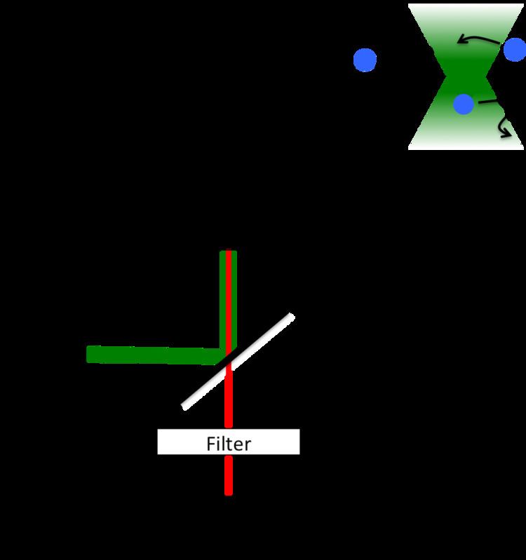
The typical FCS setup consists of a laser line (wavelengths ranging typically from 405–633 nm (cw), and from 690–1100 nm (pulsed)), which is reflected into a microscope objective by a dichroic mirror. The laser beam is focused in the sample, which contains fluorescent particles (molecules) in such high dilution, that only a few are within the focal spot (usually 1–100 molecules in one fL). When the particles cross the focal volume, they fluoresce. This light is collected by the same objective and, because it is red-shifted with respect to the excitation light it passes the dichroic mirror reaching a detector, typically a photomultiplier tube, an avalanche photodiode detector or a superconducting nanowire single-photon detector. The resulting electronic signal can be stored either directly as an intensity versus time trace to be analyzed at a later point, or computed to generate the autocorrelation directly (which requires special acquisition cards). The FCS curve by itself only represents a time-spectrum. Conclusions on physical phenomena have to be extracted from there with appropriate models. The parameters of interest are found after fitting the autocorrelation curve to modeled functional forms.

The measurement volume

The measurement volume is a convolution of illumination (excitation) and detection geometries, which result from the optical elements involved. The resulting volume is described mathematically by the point spread function (or PSF), it is essentially the image of a point source. The PSF is often described as an ellipsoid (with unsharp boundaries) of few hundred nanometers in focus diameter, and almost one micrometer along the optical axis. The shape varies significantly (and has a large impact on the resulting FCS curves) depending on the quality of the optical elements (it is crucial to avoid astigmatism and to check the real shape of the PSF on the instrument). In the case of confocal microscopy, and for small pinholes (around one Airy unit), the PSF is well approximated by Gaussians:

P S F ( r , z ) = I 0 e − 2 r 2 / ω x y 2 e − 2 z 2 / ω z 2

where I 0 is the peak intensity, r and z are radial and axial position, and ω x y and ω z are the radial and axial radii, and ω z > ω x y . This Gaussian form is assumed in deriving the functional form of the autocorrelation.

Typically ω x y is 200–300 nm, and ω z is 2–6 times larger. One common way of calibrating the measurement volume parameters is to perform FCS on a species with known diffusion coefficient and concentration (see below). Diffusion coefficients for common fluorophores in water are given in a later section.

The Gaussian approximation works to varying degrees depending on the optical details, and corrections can sometimes be applied to offset the errors in approximation.

Autocorrelation function

The (temporal) autocorrelation function is the correlation of a time series with itself shifted by time τ , as a function of τ :

G ( τ ) = ⟨ δ I ( t ) δ I ( t + τ ) ⟩ ⟨ I ( t ) ⟩ 2 = ⟨ I ( t ) I ( t + τ ) ⟩ ⟨ I ( t ) ⟩ 2 − 1

where δ I ( t ) = I ( t ) − ⟨ I ( t ) ⟩ is the deviation from the mean intensity. The normalization (denominator) here is the most commonly used for FCS, because then the correlation at τ = 0 , G(0), is related to the average number of particles in the measurement volume.

As an example, raw FCS data and its autocorrelation for freely diffusing Rhodamine 6G are shown in the figure to the right. The plot on top shows the fluorescent intensity versus time. The intensity fluctuates as Rhodamine 6G moves in and out of the focal volume. In the bottom plot is the autocorrelation on the same data. Information about the diffusion rate and concentration can be obtained using one of the models described below.

For a Gaussian illumination profile P S F ( r , z ) , the autocorrelation function is given by the general master formula

G ( τ ) = 1 ⟨ N ⟩ ⟨ exp ⁡ ( − Δ X ( τ ) 2 + Δ Y ( τ ) 2 w x y 2 − Δ Z ( τ ) 2 w z 2 ) ⟩ ,

where the vector Δ R → ( τ ) = ( Δ X ( τ ) , Δ Y ( τ ) , Δ Z ( τ ) ) denotes the stochastic displacement in space of a fluorophore after time τ . The expression is valid if the average number ⟨ N ⟩ of fluorophores in the focal volume is low and if dark states, etc., of the fluorophore can be ignored. It particular, no assumption was made on the type of diffusive motion under investigation. The formula allows for an interpretation of G ( τ ) as (i) a return probability for small beam parameters w x y , w z and (ii) the moment-generating function of | Δ R → ( τ ) | 2 if w x y , w z are varied.

Interpreting the autocorrelation function

To extract quantities of interest, the autocorrelation data can be fitted, typically using a nonlinear least squares algorithm. The fit's functional form depends on the type of dynamics (and the optical geometry in question).

Normal diffusion

The fluorescent particles used in FCS are small and thus experience thermal motions in solution. The simplest FCS experiment is thus normal 3D diffusion, for which the autocorrelation is:

G ( τ ) = G ( 0 ) 1 ( 1 + ( τ / τ D ) ) ( 1 + a − 2 ( τ / τ D ) ) 1 / 2 + G ( ∞ )

where a = ω z / ω x y is the ratio of axial to radial e − 2 radii of the measurement volume, and τ D is the characteristic residence time. This form was derived assuming a Gaussian measurement volume. Typically, the fit would have three free parameters—G(0), G ( ∞ ) , and τ D —from which the diffusion coefficient and fluorophore concentration can be obtained.

With the normalization used in the previous section, G(0) gives the mean number of diffusers in the volume <N>, or equivalently—with knowledge of the observation volume size—the mean concentration:

G ( 0 ) = 1 ⟨ N ⟩ = 1 V eff ⟨ C ⟩ ,

where the effective volume is found from integrating the Gaussian form of the measurement volume and is given by:

V eff = π 3 / 2 ω x y 2 ω z . D gives the diffusion coefficient: D = ω x y 2 / 4 τ D .

Anomalous diffusion

If the diffusing particles are hindered by obstacles or pushed by a force (molecular motors, flow, etc.) the dynamics is often not sufficiently well-described by the normal diffusion model, where the mean squared displacement (MSD) grows linearly with time. Instead the diffusion may be better described as anomalous diffusion, where the temporal dependence of the MSD is non-linear as in the power-law:

M S D = 6 D a t α

where D a is an anomalous diffusion coefficient. "Anomalous diffusion" commonly refers only to this very generic model, and not the many other possibilities that might be described as anomalous. Also, a power law is, in a strict sense, the expected form only for a narrow range of rigorously defined systems, for instance when the distribution of obstacles is fractal. Nonetheless a power law can be a useful approximation for a wider range of systems.

The FCS autocorrelation function for anomalous diffusion is:

G ( τ ) = G ( 0 ) 1 ( 1 + ( τ / τ D ) α ) ( 1 + a − 2 ( τ / τ D ) α ) 1 / 2 + G ( ∞ ) ,

where the anomalous exponent α is the same as above, and becomes a free parameter in the fitting.

Using FCS, the anomalous exponent has been shown to be an indication of the degree of molecular crowding (it is less than one and smaller for greater degrees of crowding).

Polydisperse diffusion

If there are diffusing particles with different sizes (diffusion coefficients), it is common to fit to a function that is the sum of single component forms:

G ( τ ) = G ( 0 ) ∑ i α i ( 1 + ( τ / τ D , i ) ) ( 1 + a − 2 ( τ / τ D , i ) ) 1 / 2 + G ( ∞ )

where the sum is over the number different sizes of particle, indexed by i, and α i gives the weighting, which is related to the quantum yield and concentration of each type. This introduces new parameters, which makes the fitting more difficult as a higher-dimensional space must be searched. Nonlinear least square fitting typically becomes unstable with even a small number of τ D , i s. A more robust fitting scheme, especially useful for polydisperse samples, is the Maximum Entropy Method.

Diffusion with flow

With diffusion together with a uniform flow with velocity v in the lateral direction, the autocorrelation is:

G ( τ ) = G ( 0 ) 1 ( 1 + ( τ / τ D ) ) ( 1 + a − 2 ( τ / τ D ) ) 1 / 2 × exp ⁡ [ − ( τ / τ v ) 2 × 1 1 + τ / τ D ] + G ( ∞ )

where τ v = ω x y / v is the average residence time if there is only a flow (no diffusion).

Chemical relaxation

A wide range of possible FCS experiments involve chemical reactions that continually fluctuate from equilibrium because of thermal motions (and then "relax"). In contrast to diffusion, which is also a relaxation process, the fluctuations cause changes between states of different energies. One very simple system showing chemical relaxation would be a stationary binding site in the measurement volume, where particles only produce signal when bound (e.g. by FRET, or if the diffusion time is much faster than the sampling interval). In this case the autocorrelation is:

G ( τ ) = G ( 0 ) exp ⁡ ( − τ / τ B ) + G ( ∞ )

where

τ B = ( k on + k off ) − 1

is the relaxation time and depends on the reaction kinetics (on and off rates), and:

G ( 0 ) = 1 ⟨ N ⟩ k o n k o f f = 1 ⟨ N ⟩ K

is related to the equilibrium constant K.

Most systems with chemical relaxation also show measurable diffusion as well, and the autocorrelation function will depend on the details of the system. If the diffusion and chemical reaction are decoupled, the combined autocorrelation is the product of the chemical and diffusive autocorrelations.

Triplet state correction

The autocorrelations above assume that the fluctuations are not due to changes in the fluorescent properties of the particles. However, for the majority of (bio)organic fluorophores—e.g. green fluorescent protein, rhodamine, Cy3 and Alexa Fluor dyes—some fraction of illuminated particles are excited to a triplet state (or other non-radiative decaying states) and then do not emit photons for a characteristic relaxation time τ F . Typically τ F is on the order of microseconds, which is usually smaller than the dynamics of interest (e.g. τ D ) but large enough to be measured. A multiplicative term is added to the autocorrelation to account for the triplet state. For normal diffusion:

G ( τ ) = G ( 0 ) ( 1 − F + F e − τ / τ F ) ( 1 − F ) 1 ( 1 + ( τ / τ D , i ) ) ( 1 + a − 2 ( τ / τ D , i ) ) 1 / 2 + G ( ∞ )

where F is the fraction of particles that have entered the triplet state and τ F is the corresponding triplet state relaxation time. If the dynamics of interest are much slower than the triplet state relaxation, the short time component of the autocorrelation can simply be truncated and the triplet term is unnecessary.

Common fluorescent probes

The fluorescent species used in FCS is typically a biomolecule of interest that has been tagged with a fluorophore (using immunohistochemistry for instance), or is a naked fluorophore that is used to probe some environment of interest (e.g. the cytoskeleton of a cell). The following table gives diffusion coefficients of some common fluorophores in water at room temperature, and their excitation wavelengths.

Variations of FCS

FCS almost always refers to the single point, single channel, temporal autocorrelation measurement, although the term "fluorescence correlation spectroscopy" out of its historical scientific context implies no such restriction. FCS has been extended in a number of variations by different researchers, with each extension generating another name (usually an acronym).

Spot variation fluorescence correlation spectroscopy (svFCS)

Whereas FCS is a point measurement providing diffusion time at a given observation volume, svFCS is a technique where the observation spot is varied in order to measure diffusion times at different spot sizes. The relationship between the diffusion time and the spot area is linear and could be plotted in order to decipher the major contribution of confinement. The resulting curve is called the diffusion law. This technique is used in Biology to study the plasma membrane organization on living cells.

ω x y 2 = 4 D τ D + t 0

where t 0 is the y axis intercept. In case of Brownian diffusion, t 0 = 0 . In case of a confinement due to isolated domains, t 0 > 0 whereas in case of isolated domains, t 0 < 0 .

svFCS studies on living cells and simulation papers

Sampling-Volume-Controlled Fluorescence Correlation Spectroscopy (SVC-FCS):

z-scan FCS

FCS with Nano-apertures: breaking the diffraction barrier

STED-FCS:

Fluorescence cross-correlation spectroscopy (FCCS)

FCS is sometimes used to study molecular interactions using differences in diffusion times (e.g. the product of an association reaction will be larger and thus have larger diffusion times than the reactants individually); however, FCS is relatively insensitive to molecular mass as can be seen from the following equation relating molecular mass to the diffusion time of globular particles (e.g. proteins):

τ D = 3 π ω x y 2 η 2 k T ( M ) 1 / 3

where η is the viscosity of the sample and M is the molecular mass of the fluorescent species. In practice, the diffusion times need to be sufficiently different—a factor of at least 1.6—which means the molecular masses must differ by a factor of 4. Dual color fluorescence cross-correlation spectroscopy (FCCS) measures interactions by cross-correlating two or more fluorescent channels (one channel for each reactant), which distinguishes interactions more sensitively than FCS, particularly when the mass change in the reaction is small.

Brightness analysis methods (N&B, PCH, FIDA, Cumulant Analysis)

Fluorescence cross correlation spectroscopy overcomes the weak dependence of diffusion rate on molecular mass by looking at multicolor coincidence. What about homo-interactions? The solution lies in brightness analysis. These methods use the heterogeneity in the intensity distribution of fluorescence to measure the molecular brightness of different species in a sample. Since dimers will contain twice the number of fluorescent labels as monomers, their molecular brightness will be approximately double that of monomers. As a result, the relative brightness is sensitive a measure of oligomerization. The average molecular brightness ( ⟨ ϵ ⟩ ) is related to the variance ( σ 2 ) and the average intensity ( ⟨ I ⟩ ) as follows:

⟨ ε ⟩ = σ 2 − ⟨ I ⟩ ⟨ I ⟩ = ∑ i f i ε i

Here f i and ϵ i are the fractional intensity and molecular brightness, respectively, of species i .

FRET-FCS

Another FCS based approach to studying molecular interactions uses fluorescence resonance energy transfer (FRET) instead of fluorescence, and is called FRET-FCS. With FRET, there are two types of probes, as with FCCS; however, there is only one channel and light is only detected when the two probes are very close—close enough to ensure an interaction. The FRET signal is weaker than with fluorescence, but has the advantage that there is only signal during a reaction (aside from autofluorescence).

Scanning FCS

In Scanning fluorescence correlation spectroscopy (sFCS) the measurement volume is moved across the sample in a defined way. The introduction of scanning is motivated by its ability to alleviate or remove several distinct problems often encountered in standard FCS, and thus, to extend the range of applicability of fluorescence correlation methods in biological systems.

Some variations of FCS are only applicable to serial scanning laser microscopes. Image Correlation Spectroscopy and its variations all were implemented on a scanning confocal or scanning two photon microscope, but transfer to other microscopes, like a spinning disk confocal microscope. Raster ICS (RICS), and position sensitive FCS (PSFCS) incorporate the time delay between parts of the image scan into the analysis. Also, low-dimensional scans (e.g. a circular ring)—only possible on a scanning system—can access time scales between single point and full image measurements. Scanning path has also been made to adaptively follow particles.

Spinning disk FCS and spatial mapping

Any of the image correlation spectroscopy methods can also be performed on a spinning disk confocal microscope, which in practice can obtain faster imaging speeds compared to a laser scanning confocal microscope. This approach has recently been applied to diffusion in a spatially varying complex environment, producing a pixel resolution map of a diffusion coefficient. The spatial mapping of diffusion with FCS has subsequently been extended to the TIRF system. Spatial mapping of dynamics using correlation techniques had been applied before, but only at sparse points or at coarse resolution.

Image correlation spectroscopy (ICS)

When the motion is slow (in biology, for example, diffusion in a membrane), getting adequate statistics from a single-point FCS experiment may take a prohibitively long time. More data can be obtained by performing the experiment in multiple spatial points in parallel, using a laser scanning confocal microscope. This approach has been called Image Correlation Spectroscopy (ICS). The measurements can then be averaged together.

Another variation of ICS performs a spatial autocorrelation on images, which gives information about the concentration of particles. The correlation is then averaged in time. While camera white noise does not autocorrelate over time, it does over space - this creates a white noise amplitude in the spatial autocorrelation function which must be accounted for when fitting the autocorrelation amplitude in order to find the concentration of fluorescent molecules.

A natural extension of the temporal and spatial correlation versions is spatio-temporal ICS (STICS). In STICS there is no explicit averaging in space or time (only the averaging inherent in correlation). In systems with non-isotropic motion (e.g. directed flow, asymmetric diffusion), STICS can extract the directional information. A variation that is closely related to STICS (by the Fourier transform) is k-space Image Correlation Spectroscopy (kICS).

There are cross-correlation versions of ICS as well, which can yield the concentration, distribution and dynamics of co-localized fluorescent molecules. Molecules are considered co-localized when individual fluorescence contributions are indistinguishable due to overlapping point-spread functions of fluorescence intensities.

Particle image correlation spectroscopy (PICS)

PICS is a powerful analysis tool that resolves correlations on the nanometer length and millisecond timescale. Adapted from methods of spatio-temporal image correlation spectroscopy, it exploits the high positional accuracy of single-particle tracking. While conventional tracking methods break down if multiple particle trajectories intersect, this method works in principle for arbitrarily large molecule densities and dynamical parameters (e.g. diffusion coefficients, velocities) as long as individual molecules can be identified. It is computationally cheap and robust and allows one to identify and quantify motions (e.g. diffusion, active transport, confined diffusion) within an ensemble of particles, without any a priori knowledge about the dynamics.

A particle image cross-correlation spectroscopy (PICCS) extension is available for biological processes that involve multiple interaction partners, as can observed by two-color microscopy.

FCS Super-resolution Optical Fluctuation Imaging (fcsSOFI)

Super-resolution optical fluctuation imaging (SOFI) is a super-resolution technique that achieves spatial resolutions below the diffraction limit by post-processing analysis with correlation equations, similar to FCS. While original reports of SOFI used fluctuations from stationary, blinking of fluorophores, FCS has been combined with SOFI where fluctuations are produced from diffusing probes to produce super-resolution spatial maps of diffusion coefficients. This has been applied to understand diffusion and spatial properties of porous materials, including agarose hydrogels and liquid crystals.

Total internal reflection FCS

Total internal reflection fluorescence (TIRF) is a microscopy approach that is only sensitive to a thin layer near the surface of a coverslip, which greatly minimizes background fluorescence. FCS has been extended to that type of microscope, and is called TIR-FCS. Because the fluorescence intensity in TIRF falls off exponentially with distance from the coverslip (instead of as a Gaussian with a confocal), the autocorrelation function is different.

FCS imaging using Light sheet fluorescence microscopy

Light sheet fluorescence microscopy or selective plane imaging microscopy (SPIM) uses illumination that is done perpendicularly to the direction of observation, by using a thin sheet of (laser) light. Under certain conditions, this illumination principle can be combined with fluorescence correlation spectroscopy, to allow spatially resolved imaging of the mobility and interactions of fluorescing particles such as GFP labelled proteins inside living biological samples.

Other fluorescent dynamical approaches

There are two main non-correlation alternatives to FCS that are widely used to study the dynamics of fluorescent species.

Fluorescence recovery after photobleaching (FRAP)

In FRAP, a region is briefly exposed to intense light, irrecoverably photobleaching fluorophores, and the fluorescence recovery due to diffusion of nearby (non-bleached) fluorophores is imaged. A primary advantage of FRAP over FCS is the ease of interpreting qualitative experiments common in cell biology. Differences between cell lines, or regions of a cell, or before and after application of drug, can often be characterized by simple inspection of movies. FCS experiments require a level of processing and are more sensitive to potentially confounding influences like: rotational diffusion, vibrations, photobleaching, dependence on illumination and fluorescence color, inadequate statistics, etc. It is much easier to change the measurement volume in FRAP, which allows greater control. In practice, the volumes are typically larger than in FCS. While FRAP experiments are typically more qualitative, some researchers are studying FRAP quantitatively and including binding dynamics. A disadvantage of FRAP in cell biology is the free radical perturbation of the cell caused by the photobleaching. It is also less versatile, as it cannot measure concentration or rotational diffusion, or co-localization. FRAP requires a significantly higher concentration of fluorophores than FCS.

Particle tracking

In particle tracking, the trajectories of a set of particles are measured, typically by applying particle tracking algorithms to movies.[1] Particle tracking has the advantage that all the dynamical information is maintained in the measurement, unlike FCS where correlation averages the dynamics to a single smooth curve. The advantage is apparent in systems showing complex diffusion, where directly computing the mean squared displacement allows straightforward comparison to normal or power law diffusion. To apply particle tracking, the particles have to be distinguishable and thus at lower concentration than required of FCS. Also, particle tracking is more sensitive to noise, which can sometimes affect the results unpredictably.

Two- and three- photon FCS excitation

Several advantages in both spatial resolution and minimizing photodamage/photobleaching in organic and/or biological samples are obtained by two-photon or three-photon excitation FCS.

References

Fluorescence correlation spectroscopy Wikipedia

(Text) CC BY-SA

Contents