Fast Algorithms for Multidimensional Signals

Motivation and applications

In the case of digital systems, a mathematical expressions can be used to describe the input-output relationship and an algorithm can be used to implement this relationship. Similarly, algorithms can be developed to implement different transforms such as Digital filter, Fourier transform, Histogram, Image Enhancements and etc. Direct implementation of these input-output relationships and transforms is not necessarily the most efficient way to implement those.

When people began to compute such outputs from input through direct implementation, they began to look for more efficient ways. This wiki page aims at showcasing such efficient and fast algorithms for multidimensional signals and systems. A multidimensional (M-D) signal can be modeled as a function of M independent variables, where M is greater than or equal to 2. These signals may be categorized as continuous, discrete, or mixed. A continuous signal can be modeled as a function of independent variables which range over a continuum of values, example – an audio wave travelling in space, 3-D space waves measured at different times. A discrete signal, on the other hand, can be modeled as a function defined only on a set of points, such as the set of integers. An image is the simplest example of a 2-D discrete domain signal that is spatial in nature.

In the context of Fast Algorithms, let us consider the example below:

We need to compute A which is given by

A = αγ + αδ + βγ + βδ where α,β,γ and δ are complex variables.

To compute A, we need 4 complex multiplications and 3 complex additions. The above equation can be written in its simplified form as

A = (α + β)(γ + δ)

This form requires only 1 complex multiplication and 2 complex additions.

Thus the second way of computing A is much more efficient and fast compared to the first method of computing A. This is the motivation for the evolution of the fast algorithms in the digital signal processing Field. Consequently, many of the real-world applications make use of these efficient Algorithms for fast computations.

Problem Statement and Basics

The simplest form of representing a Linear Shift Invariant system(LSI) is through its Impulse response. The output of such LSI discrete domain system is given by the convolution of its input signal and system’s impulse response. This is mathematically represented as follows:

y ( n 1 , n 2 ) = ∑ l 1 = − ∞ + ∞ ∑ l 2 = ∞ + ∞ x ( l 1 , l 2 ) h ( n 1 − l 1 , n 2 − l 2 )

where h ( n 1 , n 2 ) is the impulse response of the system.

According to the equation above to obtain the Output value at a particular point ( say y ( 0 , 0 ) ) we need to multiply several values of the input x ( l 1 , l 2 ) and Impulse Response h ( − l 1 , − l 2 ) . Of course this is dependent on the Region of Support of the input as well as the impulse response. The key point here to be noted is that we need to perform so many complex multiplications and additions to obtain 1 output value.

Assuming a 2-D input signal is of length M × M and the system's impulse response is of length N × N we need to perform M 2 N 2 number of multiplications to obtain all output values. The output can be computed efficiently if one can exploit some characteristics of the system.

We encounter a similar scenario when we have to compute the discrete Fourier Transforms of a signal of interest.

The Direct Calculation of the 2-D DFT is simply the evaluation of the double Sum

X ( k 1 , k 2 ) = ∑ n 1 = 0 N 1 − 1 ∑ n 2 = 0 N 2 − 1 x ( n 1 , n 2 ) W N 1 n 1 k 1 W N 2 n 2 k 2  for  0 ≤ k 1 ≤ N 1 − 1  and  0 ≤ k 2 ≤ N 2 − 1

 where  W N ≡ exp ( − j 2 π N )

The total number of complex multiplications and complex additions needed to evaluate this 2-D DFT by direct calculation is N 1 2 N 2 2 . This is a naive approach, however, we already know that an N-point 1-D DFT can be computed with far fewer than N 2 multiplications by using the Fast Fourier Transform (FFT) algorithm. As described in the next section we can develop Fast Fourier transforms for calculating 2-D or higher dimensional DFTs as well

Row Column Decomposition approach for the evaluation of DFT

The DFT sum X ( k 1 , k 2 ) in the previous equation can also be written in the following form

X ( k 1 , k 2 ) = ∑ n 1 = 0 N 1 − 1 [ ∑ n 2 = 0 N 2 − 1 x ( n 1 , n 2 ) W N 2 n 2 k 2 ] W N 1 n 1 k 1

Let G ( n 1 , k 2 ) denote the quantity inside the brackets and is given by:

G ( n 1 , k 2 ) = ∑ n 2 = 0 N 2 − 1 x ( n 1 , n 2 ) W N 2 n 2 k 2

X ( k 1 , k 2 ) = ∑ n 1 = 0 N 1 − 1 G ( n 1 , k 2 ) W N 1 n 1 k 2

Employing this method the DFT X can be computed as multiple 1-D DFTs. That is, each column of G can be considered as a 1-D DFT of the corresponding column of x ( n 1 = constant). And each row of X is the 1-DFT of the corresponding row of the G ( n 2 = constant). Hence we are computing the 2-D DFT by decomposing it into Row and Column DFTs.

The same principle is employed for evaluating the M-D DFT of a M - dimensional signal.

Now let's talk about the computational savings we get using this approach. It is observed that we require N 1 N 2 ( N 1 + N 2 ) complex additions and multiplications. Further, if each of these 1-D DFT is computed using a 1-D FFT, the number of complex multiplications can be further reduced to N 1 N 2 log 2 ⁡ N 1 N 2 2

Vector Radix Fast Fourier Transform

Just like the 1-D FFT, decimation in time can be achieved in the case of 2-D Signals. The 1-D DFT of a signal whose length is a power of 2, can be expressed in terms of two half-length DFTs, each of these can again be expressed as a combination of quarter length DFTs and so on.

In the case of 2-D signals we can express the ( N 1  x  N 2 ) DFT in terms of four N 1 2  x  N 2 2 DFTs (assuming N 1 and N 2 are powers of 2). For the sake of simplicity let us assume that N 1 = N 2 = N . The DFT double sum can be decomposed into four separate summations, one over those samples of x for which both n 1 and n 2 are even, one for which n 1 is even and n 2 is odd, one for which n 1 is odd and n 2 is even and the last one for which n 1 and n 2 are odd.

This is written as :

where

S 00 ( k 1 , k 2 ) ≡ ∑ m 1 = 0 N / 2 − 1 ∑ m 2 = 0 N / 2 − 1 x ( 2 m 1 , 2 m 2 ) W N 2 m 1 k 1 + 2 m 2 k 2

S 01 ( k 1 , k 2 ) ≡ ∑ m 1 = 0 N / 2 − 1 ∑ m 2 = 0 N / 2 − 1 x ( 2 m 1 , 2 m 2 + 1 ) W N 2 m 1 k 1 + 2 m 2 k 2

S 10 ( k 1 , k 2 ) ≡ ∑ m 1 = 0 N / 2 − 1 ∑ m 2 = 0 N / 2 − 1 x ( 2 m 1 + 1 , 2 m 2 ) W N 2 m 1 k 1 + 2 m 2 k 2

S 11 ( k 1 , k 2 ) ≡ ∑ m 1 = 0 N / 2 − 1 ∑ m 2 = 0 N / 2 − 1 x ( 2 m 1 + 1 , 2 m 2 + 1 ) W N 2 m 1 k 1 + 2 m 2 k 2

All the arrays S 00 S 01 S 10 and S 11 are each periodic in ( k 1 , k 2 ) with horizontal and vertical periods N 2 . Using this fact and also the fact that W N N / 2 = − 1 , we can obtain the following identities :

X ( k 1 , k 2 ) = S 00 ( k 1 , k 2 ) + S 01 ( k 1 , k 2 ) W N k 2 + S 10 ( k 1 , k 2 ) W N k 1 + S 11 ( k 1 , k 2 ) W N k 1 + k 2

X ( k 1 + N 2 , k 2 ) = S 00 ( k 1 , k 2 ) + S 01 ( k 1 , k 2 ) W N k 2 − S 10 ( k 1 , k 2 ) W N k 1 − S 11 ( k 1 , k 2 ) W N k 1 + k 2

X ( k 1 , k 2 + N 2 ) = S 00 ( k 1 , k 2 ) − S 01 ( k 1 , k 2 ) W N k 2 + S 10 ( k 1 , k 2 ) W N k 1 − S 11 ( k 1 , k 2 ) W N k 1 + k 2

X ( k 1 + N 2 , k 2 + N 2 ) = S 00 ( k 1 , k 2 ) − S 01 ( k 1 , k 2 ) W N k 2 − S 10 ( k 1 , k 2 ) W N k 1 + S 11 ( k 1 , k 2 ) W N k 1 + k 2

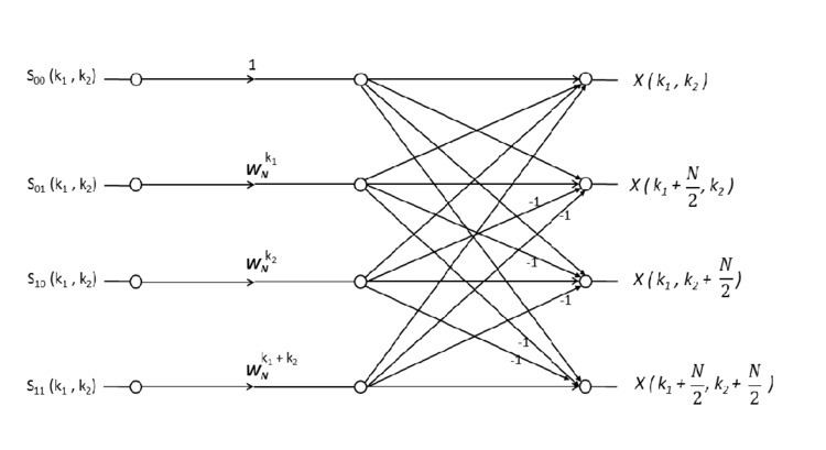
The above equation tell us how to compute the four DFT points X ( k 1 , k 2 ) X ( k 1 + N 2 , k 2 ) X ( k 1 , k 2 + N 2 )  and  X ( k 1 + N 2 , k 2 + N 2 ) for a particular value of ( k 1 , k 2 ) from the four points S 00 ( k 1 , k 2 ) S 01 ( k 1 , k 2 ) S 10 ( k 1 , k 2 )  and  S 11 ( k 1 , k 2 ) . S 00 ( k 1 , k 2 ) can be obtained by evaluating a ( N 2 × N 2 ) -point DFT (similarly other S i j can be obtained).

Thus we see that the N × N DFT can be expressed in terms of four N 2 × N 2 DFTs.

By analogy from the 1-D case, the computation depicted in the below figure is called a butterfly or more precisely r a d i x − ( 2 × 2 )  butterfly .

Each butterfly requires three complex multiplications and eight complex additions for the calculation of outputs from the inputs. And to compute all the samples of X from S 00 ( k 1 , k 2 ) , S 01 ( k 1 , k 2 ) , S 10 ( k 1 , k 2 )  and  S 11 ( k 1 , k 2 ) it requires calculations of N 2 4 butterflies.

This decimation procedure is performed log 2 ⁡ N times when N is a power of 2. Each stage of decimation consists of N 2 4 butterflies, and each butterfly involves three complex multiplications and eight complex additions and hence the number of complex multiplications that needs to be performed during the computation of an ( N × N ) -point radix ( 2 × 2 ) FFT is given by

C v e c t o r R a d i x ( 2 × 2 ) = 3 N 2 4 log 2 ⁡ N