Extension neural network

Extension Theory

Extension theory was first proposed by Cai in 1983 to solve contradictory problems. While classical mathematic is familiar with quantity and forms of objects, extension theory transforms these objects to matter-element model.

where in matter R , N is the name or type, C is its characteristics and V is the corresponding value for the characteristic. There is a corresponding example in equation 2.

where H e i g h t and W e i g h t characteristics form extension sets. These extension sets are defined by the V values which are range values for corresponding characteristics. Extension theory concerns with the extension correlation function between matter-element models like shown in equation 2 and extension sets. Extension correlation function is used to define extension space which is composed of pairs of elements and their extension correlation functions. The extension space formula is shown in equation 3.

where, A is the extension space, U is the object space, K is the extension correlation function, x is an element from the object space and y is the corresponding extension correlation function output of element x . K ( x ) maps x to a membership interval [ − ∞ , ∞ ] . Negative region represents an element not belonging membership degree to a class and positive region vice versa. If x is mapped to [ 0 , 1 ] , extension theory acts like fuzzy set theory. The correlation function can be shown with the equation 4.

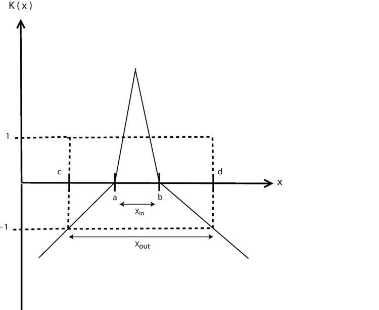
where, X i n and X o u t are called concerned and neighborhood domain and their intervals are (a,b) and (c,d) respectively. The extended correlation function used for estimation of membership degree between x and X i n , X o u t is shown in equation 5.

Extension Neural Network

Extension neural network has a neural network like appearance. Weight vector resides between the input nodes and output nodes. Output nodes are the representation of input nodes by passing them through the weight vector.

There are total number of input and output nodes are represented by n and n c , respectively. These numbers depend on the number of characteristics and classes. Rather than using one weight value between two layer nodes as in neural network, extension neural network architecture has two weight values. In extension neural network architecture, for instance i , x i j p is the input which belongs to class p and o i k is the corresponding output for class k . The output o i k is calculated by using extension distance as shown in equation 6.

Estimated class is found through searching for the minimum extension distance among the calculated extension distance for all classes as summarized in equation 7, where k ∗ is the estimated class.

Learning Algorithm

Each class is composed of ranges of characteristics. These characteristics are the input types or names which come from matter-element model. Weight values in extension neural network represent these ranges. In the learning algorithm, first weights are initialized by searching for the maximum and minimum values of inputs for each class as shown in equation 8

where, i is the instance number and j is represents number of input. This initialization provides classes' ranges according to given training data.

After maintaining weights, center of clusters are found through the equation 9.

Before learning process begins, predefined learning performance rate is given as shown in equation 10

where, N m is the misclassified instances and N p is the total number of instances. Initialized parameters are used to classify instances with using equation 6. If the initialization is not sufficient due to the learning performance rate, training is required. In the training step weights are adjusted to classify training data more accurately, therefore reducing learning performance rate is aimed. In each iteration, E τ is checked to control if required learning performance is reached. In each iteration every training instance is used for training.
Instance i , belongs to class p is shown by:

X i p = { x i 1 p , x i 2 p , . . . , x i n p }

1 ≤ p ≤ n c

Every input data point of X i p is used in extension distance calculation to estimate the class of X i p . If the estimated class k ∗ = p then update is not needed. Whereas, if k ∗ ≠ p then update is done. In update case, separators which show the relationship between inputs and classes, are shifted proportional to the distance between the center of clusters and the data points.
The update formula:

z p j n e w = z p j o l d + η ( x i j p − z p j o l d )
z k ∗ j n e w = z k ∗ j o l d − η ( x i j p − z k ∗ j o l d )
w p j L ( n e w ) = w p j L ( o l d ) + η ( x i j p − z p j o l d )
w p j U ( n e w ) = w p j U ( o l d ) + η ( x i j p − z p j o l d )
w k ∗ j L ( n e w ) = w k ∗ j L ( o l d ) − η ( x i j p − z k ∗ j o l d )
w k ∗ j U ( n e w ) = w k ∗ j U ( o l d ) − η ( x i j p − z k ∗ j o l d )

To classify the instance i accurately, separator of class p for input j moves close to data-point of instance i , whereas separator of class k ∗ for input j moves far away. In the above image, an update example is given. Assume that instance i belongs to class A, whereas it is classified to class B because extension distance calculation gives out E D A > E D B . After the update, separator of class A moves close to the data-point of instance i whereas separator of class B moves far away. Consequently, extension distance gives out E D B > E D A , therefore after update instance i is classified to class A.