Edgeworth series

Gram–Charlier A series

The key idea of these expansions is to write the characteristic function of the distribution whose probability density function F is to be approximated in terms of the characteristic function of a distribution with known and suitable properties, and to recover F through the inverse Fourier transform.

We examine a continuous random variable. Let f be the characteristic function of its distribution whose density function is F, and κ r its cumulants. We expand in terms of a known distribution with probability density function Ψ, characteristic function ψ, and cumulants γ r . The density Ψ is generally chosen to be that of the normal distribution, but other choices are possible as well. By the definition of the cumulants, we have (see Wallace, 1958)

which gives the following formal identity:

By the properties of the Fourier transform, ( i t ) r ψ ( t ) is the Fourier transform of ( − 1 ) r [ D r Ψ ] ( − x ) , where D is the differential operator with respect to x. Thus, after changing x with − x on both sides of the equation, we find for F the formal expansion

If Ψ is chosen as the normal density with mean and variance as given by F, that is, mean μ = κ 1 and variance σ 2 = κ 2 , then the expansion becomes

since γ r = 0 for all r >2 as higher cumulants of the normal distribution are 0. By expanding the exponential and collecting terms according to the order of the derivatives, we arrive at the Gram–Charlier A series. If we include only the first two correction terms to the normal distribution, we obtain

with H 3 ( x ) = x 3 − 3 x and H 4 ( x ) = x 4 − 6 x 2 + 3 (these are Hermite polynomials).

Note that this expression is not guaranteed to be positive, and is therefore not a valid probability distribution. The Gram–Charlier A series diverges in many cases of interest—it converges only if F ( x ) falls off faster than exp ⁡ ( − ( x 2 ) / 4 ) at infinity (Cramér 1957). When it does not converge, the series is also not a true asymptotic expansion, because it is not possible to estimate the error of the expansion. For this reason, the Edgeworth series (see next section) is generally preferred over the Gram–Charlier A series.

The Edgeworth series

Edgeworth developed a similar expansion as an improvement to the central limit theorem. The advantage of the Edgeworth series is that the error is controlled, so that it is a true asymptotic expansion.

Let {Z_i} be a sequence of independent and identically distributed random variables with mean μ and variance σ², and let X_n be their standardized sums:

Let F_n denote the cumulative distribution functions of the variables X_n. Then by the central limit theorem,

for every x, as long as the mean and variance are finite.

Now assume that the random variables X_i have mean μ, variance σ², and higher cumulants κ_r=σ^rλ_r. If we expand in terms of the standard normal distribution, that is, if we set

then the cumulant differences in the formal expression of the characteristic function f_n(t) of F_n are

The Edgeworth series is developed similarly to the Gram–Charlier A series, only that now terms are collected according to powers of n. Thus, we have

where P_j(x) is a polynomial of degree 3j. Again, after inverse Fourier transform, the density function F_n follows as

The first five terms of the expansion are

Here, Φ^(j)(x) is the j-th derivative of Φ(·) at point x. Remembering that the derivatives of the density of the normal distribution are related to the normal density by ϕ⁽ⁿ⁾(x)=(-1)ⁿH_n(x)ϕ(x), (where H_n is the Hermite polynomial of order n), this explains the alternative representations in terms of the density function. Blinnikov and Moessner (1998) have given a simple algorithm to calculate higher-order terms of the expansion.

Note that in case of a lattice distributions (which have discrete values), the Edgeworth expansion must be adjusted to account for the discontinuous jumps between lattice points.

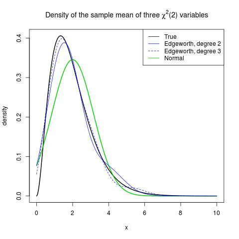
Illustration: density of the sample mean of three χ 2 {\displaystyle \chi ^{2}}

Take X i ∼ χ 2 ( k = 2 ) i = 1 , 2 , 3 and the sample mean X ¯ = 1 3 ∑ i = 1 3 X i .

We can use several distributions for X ¯ :

Disadvantages of the Edgeworth expansion

Edgeworth expansions can suffer from a few issues: