Dolinar receiver

Digital Communication with Phase Modulation of Coherent States

In a similar way that digital information can be transmitted by modulating the frequency or amplitude of electromagnetic waves, digital information can be encoded within the phase of coherent light.

Consider two coherent states, { ∣ α ⟩ , ∣ − α ⟩ } , where α is a complex vector within the phase space of a quantum harmonic oscillator such that ∣ α ∣ 2 = ⟨ n ⟩ , and ⟨ n ⟩ is the average number of photons in the state and is related to the intensity of the light. The phase angle between the ∣ α ⟩ and ∣ − α ⟩ states is π .

Binary digital communication can be achieved by sending, for instance, state ∣ α ⟩ to represent 0, and ∣ − α ⟩ to represent 1. This is known as binary phase-shift keying.

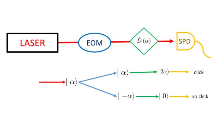
A simple example of a device that could transmit the binary coherent states is a switchable laser and an electo-optic modulator (EOM) that applies either a 0 or π phase shift on the laser pulse to send either a 0 or 1. Pulses of light defined to be in the ∣ α ⟩ state the enter the EOM. If a 0 is required to be transmitted with that pulse, the EOM does nothing and applies no phase shift. If a 1 is desired, the EOM applies a π phase shift to the pulse to prepare the outgoing ∣ − α ⟩ state from the incoming ∣ α ⟩ state.

Non-Orthogonality of Coherent States

In ideal digital communication, there is no ambiguity between when a 0 is sent and when a 1 is sent. However, if information is being transmitted via phase encoding in optical coherent states, there is no way to perfectly distinguish between any two coherent states,. This is because coherent states are not orthogonal to each other. For any two coherent states { ∣ α ⟩ , ∣ β ⟩ } it is always true that ⟨ α ∣ β ⟩ ≠ 0 . The minimum error probability, P H , assuming that there is an equally likely chance of sending either ∣ α ⟩ or ∣ β ⟩ , is given by

In the case of binary coherent state communication, where we have the two states { ∣ α ⟩ , ∣ − α ⟩ } with equal amplitudes but π out of phase with each other, the overlap between the two states is equal to

The minimum probability of error to distinguish between binary coherent states becomes,

As the average number of photons ∣ α ∣ 2 becomes very large, the minimum error becomes very small. However, for low photon numbers, the two states become less distinguishable and the error closer approaches the maximum of 50%. This inherent, fundamental source of error due to the quantum nature of the coherent state poses limits to the discrimination of low-intensity coherent states.

Kennedy Receiver

The Kennedy receiver is a device that can distinguish between binary coherent states. It operates on a basic level by first displacing the incoming state by α and the resulting state is sent to a single-photon detector (SPD), such as a photomultiplier tube or an avalanche photodiode. If the incoming state was ∣ α ⟩ , then the resultant state is,

where D ^ ( α ) is the displacement operator that displaces any coherent state by α . The displacement can be performed by interference at a beam splitter with another coherent light source of the state ∣ α ⟩ . If the incoming state is ∣ − α ⟩ , then the state becomes,

where ∣ 0 ⟩ represents the vacuum state, i.e. ∣ α ∣ 2 = 0 . One of the two final states, { ∣ 2 α ⟩ , ∣ 0 ⟩ } , then reaches the SPD. If the ∣ 2 α ⟩ state enters the detector, the SPD will most likely count a photon. If the final state is ∣ 0 ⟩ , the vacuum, there is nothing to detect, and the SPD will ideally not count a photon. Therefore, if a photon was counted, the best guess is that the original state was ∣ α ⟩ . If there is nothing, then it is safe to assume the original state was ∣ − α ⟩ .

However, it is not guaranteed that a final state of ∣ 2 α ⟩ will cause the SPD to count a photon, even if the SPD were perfect. Due to the Poissonian distribution of photons in a coherent state, there is a chance that no photons may be detected no matter how large the average number of photons is. The probability of detecting no photons with the ∣ 2 α ⟩ state, P 0 , is given by the Poissonian probability to get zero photons with average number of photons equal to 4 ∣ α ∣ 2 ,

Therefore, if the SPD detects no photons, it is not certain which state was sent. The error of guessing wrong is equal to the probability P 2 α that the ∣ α ⟩ state was sent, which is 50% as it is assumed either state is equally likely to be sent, times the probability that a zero detection result can occur when the displaced state is ∣ 2 α ⟩ . The probability of error P ϵ becomes,

By displacing the incoming states, counting photons, and thinking about what was the most likely input state given the detection results, the error in discriminating between the binary coherent states can be improved.

Principles of Operation

The Dolinar receiver expands upon the Kennedy receiver to decrease the probability of error at the cost of higher complexity. In order to operate, the Donlinar receiver needs to be sent multiple copies of the input state, or the coherent input state is split up into multiple lower-amplitude states with different detector arrival times. This can be achieved by using a series of low-reflectance beam splitters, for instance.

The Dolinar receiver also makes use of an adaptive displacement mechanism, one that can quickly change from either D ^ ( α ) or D ^ ( − α ) . If using interference from a reference state at a beam splitter to achieve the displacement, the reference state must change between ∣ α ⟩ and ∣ − α ⟩ . An EOM can be used to change the phase of the reference state by π as needed.

The unique feature of the Dolinar receiver is the feedback from the detector and the displacement mechanism in between arrivals of the input state copies. Counting either zero photons or one or more photons with the SPD does not give complete information about the input state. Rather, whether or not a photon was counted gives some information about the state, and a hypothesis can be proposed based on the information from the SPD. With the Kennedy receiver, the displacement is fixed at either D ^ ( α ) or D ^ ( − α ) , and depending on which displacement is used and if a photon is counted or not, a best hypothesis as to the nature of the input state can be put forth. For example, if the displacement of the Kennedy receiver is set to be D ^ ( α ) , then it can be said the Kennedy receiver is testing the hypothesis that the input state was ∣ − α ⟩ . If no photons are counted, it is most likely that the hypothesis was correct and that the input state was displaced to vacuum. If one or more photons are counted, it is known that the guess was wrong as the input state was not displaced to vacuum.

The feedback of the Donlinar receiver works by switching the displacement if there was a photon counted but the before the next copy of the input state arrives. If no photons are detected, the displacement remains unchanged for the next arrival of a copy. For each no count result, it becomes more and more likely that the state copies are being displaced to vacuum and the certainty of the hypothesis increases. On the whole, the history of the detection results in conjunction with their corresponding displacements can give more and more complete information about the most likely identity of the input state.

As an example, suppose before the first copy of the input state arrives, the receiver is set to test for ∣ − α ⟩ by setting the displacement to D ^ ( α ) . At this point, any hypothesis is limited by a 50% chance of guessing the input state on sheer luck alone, and thus the choice is arbitrary. However, suppose the input state is ∣ α ⟩ sent, and the displacement does not shift the state to vacuum. As is most likely, now suppose the SPD detects a photon. It is now known that the hypothesis is wrong, and the displacement is switched to D ^ ( − α ) before the next copy arrives. Now the next copy is displaced to vacuum, and there are no photons counted by the SPD. The displacement remains unchanged, and will remain unchanged for each copy of the input state that is displaced and counted by the SPD. Which each no count result, the hypothesis becomes stronger. If the ∣ − α ⟩ was sent initially, then the displacement would never change, and each lack of photon counts reinforces the initial arbitrary guess.

Another example can illustrate the potential error correction the feedback provides. Suppose the same setup as before, except that on the first detection trial no photons are detected, as is possible for the displaced ∣ 2 α ⟩ state. The receiver will not change the displacement, and the next copy of the input state will be again displaced to ∣ 2 α ⟩ . However, two no count results in a row is unlikely given the ∣ 2 α ⟩ state entering the SPD. It is most likely on the second or third pass the SPD will detect a photon and switch the displacement, after which there will be no more photon counts. As before, each lack of counted photons after a displacement switch reinforces the hypothesis that the original guess was incorrect.

The probability of N consecutive lack of photon counts for the { ∣ 2 α ⟩ , ∣ − 2 α ⟩ } displaced states grows as N products of the probability P 0 ,

Thus, the more copies of the input state being tested reduces the chance of misidentifying the input state. While more complex than the Kennedy receiver and requiring multiple copies of the input state, the Dolinar receiver's adaptive feedback offers a mechanism to reduce the chances of a hypothesis being wrong. Further, the Dolinar receiver shows more robustness against dark counts, a real-life phenomenon where SPDs can count a photon even if there is nothing, i.e. vacuum, to detect. If the detector counts a photon even when the hypothesis is correct and the input state copy was displaced to vacuum, the displacement will switch and there is a likely chance another photon will be detected on the next pass, switching the displacement back, where there will be a less likely chance to detect photons for future detection. As long as the rate of dark counts is not too high, the overall history of detection results can give a likely picture as to the nature of the original input state.

Experimental Example

An experiment using principles from the Dolinar receiver has recently been performed. In this experiment, there are four possible input states instead of two, { ∣ α ⟩ , ∣ i α ⟩ , ∣ − α ⟩ , ∣ − i α ⟩ } , each π 2 out of phase with each other. Two bits of information is encoded into each state using a method known as quadrature phase-shift keying. While the four coherent input states, being only π 2 out of phase with each other and thus more crowded in phase space, are more difficult to distinguish from each other than binary coherent states, each input state can relay more information. Because there are more input states, there are more hypothesis to test, and there are four displacements to perform in order to try to displace the input state to vacuum.

In this experiment, multiple copies of the input state are not sent to the receiver. In order to make multiple adaptive measurements, the input state is divided into ten copies, and each copy is displaced and measured in series. If no photons are detected after displacing a copy, the next displacement remains the same and another reading is taken with a detector. If a photon is detected, the next displacement may change to test a different hypothesis. However, a new hypothesis is not chosen at random. Rather, after a displacement and detection result, a deliberate decision is made on the new hypothesis given the total history of displacements and detection results using Bayesian inference. This ensures that each of the ten guesses are made as best as possible.

This awareness of the history of detection results provides robustness against dark counts inherent in the feedback technique of the Dolinar receiver. If after three displacements no photons are detected but on the fourth a photon is counted, the results of Bayesian interference may suggest that the hypothesis is still correct and the displacement may not change. If after a few more detection results no more photons are counted, it may be strongly inferred that the earlier photon count was the result of noise and that the hypothesis is still most likely correct.