
 | ||
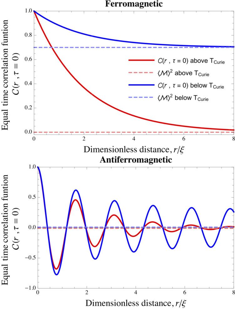
In statistical mechanics, the correlation function is a measure of the order in a system, as characterized by a mathematical correlation function. Correlation functions describe how microscopic variables, such as spin and density, at different positions are related. More specifically, correlation functions quantify how microscopic variables co-vary with one another on average across space and time. A classic example of such spatial correlations is in ferro- and antiferromagnetic materials, where the spins prefer to align parallel and antiparallel with their nearest neighbors, respectively. The spatial correlation between spins in such materials is shown in the figure to the right.
Contents
- Definitions
- Equilibrium equal time spatial correlation functions
- Equilibrium equal position temporal correlation functions
- Generalization beyond equilibrium correlation functions
- Measuring correlation functions
- Time evolution of correlation functions
- The connection between phase transitions and correlation functions
- Magnetism
- Radial distribution functions
- Higher order correlation functions
- References
Definitions
The most common definition of a correlation function is the canonical ensemble (thermal) average of the scalar product of two random variables,
Here the brackets,
Equilibrium equal-time (spatial) correlation functions
Often, one is interested in solely the spatial influence of a given random variable, say the direction of a spin, on its local environment, without considering later times,
Often, one omits the reference time,
where, again, the choice of whether to subtract the uncorrelated variables differs among fields. The Radial distribution function is an example of an equal-time correlation function where the uncorrelated reference is generally not subtracted. Other equal-time spin-spin correlation functions are shown on this page for a variety of materials and conditions.
Equilibrium equal-position (temporal) correlation functions
One might also be interested in the temporal evolution of microscopic variables. In other words, how the value of a microscopic variable at a given position and time,
Assuming equilibrium (and thus time invariance of the ensemble) and averaging over all sites in the sample gives a simpler expression for the equal-position correlation function as for the equal-time correlation function:
The above assumption may seem non-intuitive at first: how can an ensemble which is time-invariant have a non-uniform temporal correlation function? Temporal correlations remain relevant to talk about in equilibrium systems because a time-invariant, macroscopic ensemble can still have non-trivial temporal dynamics microscopically. One example is in diffusion. A single-phase system at equilibrium has a homogeneous composition macroscopically. However, if one watches the microscopic movement of each atom, fluctuations in composition are constantly occurring due to the quasi-random walks taken by the individual atoms. Statistical mechanics allows one to make insightful statements about the temporal behavior of such fluctuations of equilibrium systems. This is discussed below in the section on the temporal evolution of correlation functions and Onsager's regression hypothesis.
Generalization beyond equilibrium correlation functions
All of the above correlation functions have been defined in the context of equilibrium statistical mechanics. However, it is possible to define correlation functions for systems away from equilibrium. Examining the general definition of
One can also define averages over states for systems perturbed slightly from equilibrium. See, for example, http://xbeams.chem.yale.edu/~batista/vaa/node56.html
Measuring correlation functions
Correlation functions are typically measured with scattering experiments. For example, x-ray scattering experiments directly measure electron-electron equal-time correlations. From knowledge of elemental structure factors, one can also measure elemental pair correlation functions. See Radial distribution function for further information. Equal-time spin–spin correlation functions are measured with neutron scattering as opposed to x-ray scattering. Neutron scattering can also yield information on pair correlations as well. For systems composed of particles larger than about one micrometer, optical microscopy can be used to measure both equal-time and equal-position correlation functions. Optical microscopy is thus common for colloidal suspensions, especially in two dimensions.
Time evolution of correlation functions
In 1931, Lars Onsager proposed that "the regression of microscopic thermal fluctuations at equilibrium follows the macroscopic law of relaxation of small non-equilibrium disturbances." This is known as the Onsager regression hypothesis. As the values of microscopic variables separated by large timescales,
The connection between phase transitions and correlation functions
Continuous phase transitions, such as order-disorder transitions in metallic alloys and ferromagnetic-paramagnetic transitions, involve a transition from an ordered to a disordered state. In terms of correlation functions, the equal-time correlation function is non-zero for all lattice points below the critical temperature, and is non-negligible for only a fairly small radius above the critical temperature. As the phase transition is continuous, the length over which the microscopic variables are correlated,
Magnetism
In a spin system, the equal-time correlation function is especially well-studied. It describes the canonical ensemble (thermal) average of the scalar product of the spins at two lattice points over all possible orderings:
Even in a magnetically disordered phase, spins at different positions are correlated, i.e., if the distance r is very small (compared to some length scale
where r is the distance between spins, and d is the dimension of the system, and
As the temperature is lowered, thermal disordering is lowered, and in a continuous phase transition the correlation length diverges, as the correlation length must transition continuously from a finite value above the phase transition, to infinite below the phase transition:
with another critical exponent
This power law correlation is responsible for the scaling, seen in these transitions. All exponents mentioned are independent of temperature. They are in fact universal, i.e. found to be the same in a wide variety of systems.
Radial distribution functions
One common correlation function is the radial distribution function which is seen often in statistical mechanics. The correlation function can be calculated in exactly solvable models (one-dimensional Bose gas, spin chains, Hubbard model) by means of Quantum inverse scattering method and Bethe ansatz. In an isotropic XY model, time and temperature correlations were evaluated by Its, Korepin, Izergin & Slavnov.
Higher order correlation functions
Higher-order correlation functions involve multiple reference points, and are defined through a generalization of the above correlation function by simply taking the expected value of the product of more than two random variables:
However, such higher order correlation functions are relatively difficult to interpret and measure. For example, in order to measure the higher-order analogues of pair distribution functions, coherent x-ray sources are needed. Both the theory of such analysis and the experimental measurement of the needed X-ray cross-correlation functions are areas of active research.