Continuous time quantum walk

Introduction

Ever since the advent of quantum mechanics and the discovery by Shor of how to achieve factorization of large semi-primes efficiently (polynomial time) using quantum computation, scientists have been intrigued by the realm of possibilities. In many cases where the quantum algorithms are derived for problems, the complexity of the algorithms are faster than their classical counterpart. Some of these include Shor's factorization algorithm, which is exponentially faster than known classical factoring algorithms, and Grover's searching algorithms, which is polynomially faster than any possible black-box classical algorithm. Many of these algorithms use (or can be modified to use) the concept of quantum fourier transform.

In recent times, some scientists have decided to propose a new form of looking at quantum computation algorithms. The reason is that many classical algorithms are based on (classical) random walks. This led to the intuitive question of whether a "quantum random walk" (or simply "quantum walk") could be proposed. One such model of a quantum walk is the Continuous-time quantum walk (CTQW) proposed by E. Farhi et al. There are a number of variations to representing a CTQW, but we follow the definition below.

Mathematical definition

A continuous-time quantum walk (CTQW) on a graph G = (V,E), where V is the set of vertices (nodes) and E is the set of edges connecting the nodes, is defined as follows:
Let A be the |V| × |V| adjacency matrix of G with elements

and D be the |V| × |V| degree matrix of G (for which the diagonal entry corresponding to vertex v is degree(v)), and let L = D - A, be the corresponding Laplacian matrix which is positive semidefinite. The continuous-time quantum walk on the graph G is then defined by the unitary matrix

where i is the imaginary unit and t ∈ R . The probability of a walk starting at vertex u ending up at vertex v at time t is given by | ⟨ v | U ( t ) | u ⟩ | 2 . Consequently starting from the quantum state | ψ 0 ⟩ and performing a quantum walk for time t will result in the new state | ψ t ⟩ = U ( t ) | ψ 0 ⟩ and measuring will thus localize the walk in vertex v with the probability | ⟨ v | U ( t ) | ψ 0 ⟩ | 2 .

Quantum walk

To discuss the quantum walk, it is useful to define the more familiar topic of (classical) random walk (CRW). The random walk is well-defined in random processes with the Markov process model.

Classical random walk (CRW)

Here, a graph is traversed in an order that predicts the probability of being at a node v in time t given that the walk starts from a node u in the graph. To elaborate this concept, consider the case of a classical walk on a line. Assume a person, John, stands at the origin of a straight line and he has a fair coin. John wants to exhibit a random walk in which the probability of moving a step to the left or right is equal (=1/2). John flips his coin and the outcome dictates where he goes next. If the outcome is head (H), he takes one step to the right and if it is tail (T), he takes one step to the left. Following this rule, then the probability of John being at position d after N steps can be shown to be

Since John has a fair coin, the average of his distribution (where he's expected to be on the average) is the origin (position 0), and the standard deviation can be shown to be N . A table showing the probability of this distribution for up to the fourth step is shown below:

Continuous-time quantum walk (CTQW)

Now, the fair coin in John's possession is replaced with a qubit. This qubit is defined in terms of states | ↓ ⟩ and | ↑ ⟩ different from the | 0 ⟩ , | 1 ⟩ basis. Next, a Hadamard operation is applied to the initial state. A Hadamard on the up state will give a superposition of up and down as follows

and

After applying the Hadamard operator, the spin-1/2 rotation in the z-direction is applied, thereby stepping left or right based on the resulting state. Overall, the applied operator becomes

where σ z is the Pauli-Z operator and p ^ is the momentum operator of the qubit particle. This evolving operator in the CTQW is applied N times to the resulting qubit states. When the initial state representing the origin of the line is chosen to be 1 2 | ↑ ⟩ + 1 2 | ↓ ⟩ , the standard deviation is shown to be approximately 3 5 N which is in quadratic form of the standard deviation from classical algorithm. In this case the probability of being at position d after N steps is different from the classical case as depicted below: Note that the description employs a discrete-time quantum walk, but it provides an intuitive use on the graph problem for the continuous-time quantum walk where the Hamiltonian evolves the state of the system at any given time.

Difference between CTQW and CRW

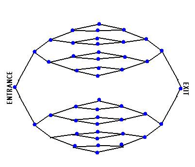
Farhi et al. showed that on a symmetric graph known as G 4 , which consists of two binary trees of depth four merged at their leaf nodes, it is possible for a quantum walk to achieve exponential speed-up over its classical counterpart.

It could be deduced that the probability of reaching the EXIT node from the ENTRANCE node of a G n is less than 2 − n , but in the quantum case, the limiting distribution probability is at least ( 2 n + 1 ) − 1 . This is a tremendous increase, but it only states that the time to reach the EXIT is faster as contrasted from the algorithmic speedup. However, it was later shown by the same author that indeed an exponential algorithmic speedup can be achieved by the quantum walk.

It is also important to note that the quantum walk 'collapses' to a classical random walk with the degree of decoherence. It is possible to obtain the classical if one measures the positions in the quantum work at every step. In other words, the inability to have superposition restricts the classical domain of walks in graph theory.

Potential applications

The area of CTQW as well as discrete-time quantum walk has given additional insight on how to achieve quantum computation. It is an area of research that is still captivating interest and a number of algorithm using CTQW has been proposed. The three main applications to date are

1. Quantum search algorithm
2. Graph Traversal problem
3. Quantum scattering NAND-tree

In each case, the algorithmic speedup is not different from what was expected in existing quantum algorithms like the Grover search algorithm that takes O ( N ) .