Confidence distribution

The history of CD concept

Neyman (1937) introduced the idea of "confidence" in his seminal paper on confidence intervals which clarified the frequentist repetition property. According to Fraser, the seed (idea) of confidence distribution can even be traced back to Bayes (1763) and Fisher (1930). Some researchers view the confidence distribution as "the Neymanian interpretation of Fishers fiducial distribution", which was "furiously disputed by Fisher". It is also believed that these "unproductive disputes" and Fisher's "stubborn insistence" might be the reason that the concept of confidence distribution has been long misconstrued as a fiducial concept and not been fully developed under the frequentist framework. Indeed, the confidence distribution is a purely frequentist concept with a purely frequentist interpretation, and it also has ties to Bayesian inference concepts and the fiducial arguments.

Classical definition

Classically, a confidence distribution is defined by inverting the upper limits of a series of lower sided confidence intervals. In particular,

For every α in (0, 1), let (−∞, ξ_n(α)] be a 100α% lower-side confidence interval for θ, where ξ_n(α) = ξ_n(X_n,α) is continuous and increasing in α for each sample X_n. Then, H_n(•) = ξ_n⁻¹(•) is a confidence distribution for θ.

Efron stated that this distribution "assigns probability 0.05 to θ lying between the upper endpoints of the 0.90 and 0.95 confidence interval, etc." and "it has powerful intuitive appeal". In the classical literature, the confidence distribution function is interpreted as a distribution function of the parameter θ, which is impossible unless fiducial reasoning is involved since, in a frequentist setting, the parameters are fixed and nonrandom.

To interpret the CD function entirely from a frequentist viewpoint and not interpret it as a distribution function of a (fixed/nonrandom) parameter is one of the major departures of recent development relative to the classical approach. The nice thing about treating confidence distribution as a purely frequentist concept (similar to a point estimator) is that it is now free from those restrictive, if not controversial, constraints set forth by Fisher on fiducial distributions.

The modern definition

The following definition applies; Θ is the parameter space of the unknown parameter of interest θ, and χ is the sample space corresponding to data X_n={X₁, ..., X_n}:

A function H_n(•) = H_n(X_n, •) on χ × Θ → [0, 1] is called a confidence distribution (CD) for a parameter θ, if it follows two requirements:

(R1) For each given X_n ∈ χ, H_n(•) = H_n(X_n, •) is a continuous cumulative distribution function on Θ;

(R2) At the true parameter value θ = θ₀, H_n(θ₀) ≡ H_n(X_n, θ₀), as a function of the sample X_n, follows the uniform distribution U[0, 1].

Also, the function H is an asymptotic CD (aCD), if the U[0, 1] requirement is true only asymptotically and the continuity requirement on H_n(•) is dropped.

In nontechnical terms, a confidence distribution is a function of both the parameter and the random sample, with two requirements. The first requirement (R1) simply requires that a CD should be a distribution on the parameter space. The second requirement (R2) sets a restriction on the function so that inferences (point estimators, confidence intervals and hypothesis testing, etc.) based on the confidence distribution have desired frequentist properties. This is similar to the restrictions in point estimation to ensure certain desired properties, such as unbiasedness, consistency, efficiency, etc.

A confidence distribution derived by inverting the upper limits of confidence intervals (classical definition) also satisfies the requirements in the above definition and this version of the definition is consistent with the classical definition.

Unlike the classical fiducial inference, more than one confidence distributions may be available to estimate a parameter under any specific setting. Also, unlike the classical fiducial inference, optimality is not a part of requirement. Depending on the setting and the criterion used, sometimes there is a unique "best" (in terms of optimality) confidence distribution. But sometimes there is no optimal confidence distribution available or, in some extreme cases, we may not even be able to find a meaningful confidence distribution. This is not different from the practice of point estimation.

Examples

Example 1: Normal Mean and Variance

Suppose a normal sample X_i ~ N(μ, σ²), i = 1, 2, ..., n is given.

(1) Variance σ² is known

Both the functions H Φ ( μ ) and H t ( μ ) given by

H Φ ( μ ) = Φ ( n ( μ − X ¯ ) σ ) , and H t ( μ ) = F t n − 1 ( n ( μ − X ¯ ) s ) ,

satisfy the two requirements in the CD definition, and they are confidence distribution functions for μ. Here, Φ is the cumulative distribution function of the standard normal distribution, and F t n − 1 is the cumulative distribution function of the student t n − 1 distribution. Furthermore,

H A ( μ ) = Φ ( n ( μ − X ¯ ) s )

satisfies the definition of an asymptotic confidence distribution when n→∞, and it is an asymptotic confidence distribution for μ. The uses of H t ( μ ) and H A ( μ ) are equivalent to state that we use N ( X ¯ , σ 2 ) and N ( X ¯ , s 2 ) to estimate μ , respectively.

(2) Variance σ² is unknown

For the parameter μ, since H Φ ( μ ) involves the unknown parameter σ and it violates the two requirements in the CD definition, it is no longer a "distribution estimator" or a confidence distribution for μ. However, H t ( μ ) is still a CD for μ and H A ( μ ) is an aCD for μ.

For the parameter σ², the sample-dependent cumulative distribution function

H χ 2 ( θ ) = 1 − F χ n − 1 2 ( ( n − 1 ) s 2 / θ )

is a confidence distribution function for σ². Here, F χ n − 1 2 is the cumulative distribution function of the student χ n − 1 2 distribution .

In the case when the variance σ² is known, H Φ ( μ ) = Φ ( n ( μ − X ¯ ) σ ) is optimal in terms of producing the shortest confidence intervals at any given level. In the case when the variance σ² is unknown, H t ( μ ) = F t n − 1 ( n ( μ − X ¯ ) s ) is an optimal confidence distribution for μ.

Example 2: Bivariate normal correlation

Let ρ denotes the correlation coefficient of a bivariate normal population. It is well known that Fisher's z defined by the Fisher transformation:

z = 1 2 ln ⁡ 1 + r 1 − r

has the limiting distribution N ( 1 2 ln ⁡ 1 + ρ 1 − ρ , 1 n − 3 ) with a fast rate of convergence, where r is the sample correlation and n is the sample size.

The function

H n ( ρ ) = 1 − Φ ( n − 3 ( 1 2 ln ⁡ 1 + r 1 − r − 1 2 ln ⁡ 1 + ρ 1 − ρ ) )

is an asymptotic confidence distribution for ρ.

Confidence interval

From the CD definition, it is evident that the interval ( − ∞ , H n − 1 ( 1 − α ) ] , [ H n − 1 ( α ) , ∞ ) and [ H n − 1 ( α / 2 ) , H n − 1 ( 1 − α / 2 ) ] provide 100(1 − α)%-level confidence intervals of different kinds, for θ, for any α ∈ (0, 1). Also [ H n − 1 ( α 1 ) , H n − 1 ( 1 − α 2 ) ] is a level 100(1 − α₁ − α₂)% confidence interval for the parameter θ for any α₁ > 0, α₂ > 0 and α₁ + α₂ < 1. Here, H n − 1 ( β ) is the 100β% quantile of H n ( θ ) or it solves for θ in equation H n ( θ ) = β . The same holds for an aCD, where the confidence level is achieved in limit.

Point estimation

Point estimators can also be constructed given a confidence distribution estimator for the parameter of interest. For example, given H_n(θ) the CD for a parameter θ, natural choices of point estimators include the median M_n = H_n⁻¹(1/2), the mean θ ¯ n = ∫ − ∞ ∞ t d H n ( t ) , and the maximum point of the CD density

θ ^ n = arg ⁡ max θ h n ( θ ) , h n ( θ ) = H n ′ ( θ ) .

Under some modest conditions, among other properties, one can prove that these point estimators are all consistent.

Hypothesis testing

One can derive a p-value for a test, either one-sided or two-sided, concerning the parameter θ, from its confidence distribution H_n(θ). Denote by the probability mass of a set C under the confidence distribution function p s ( C ) = H n ( C ) = ∫ C d H ( θ ) . This p_s(C) is called "support" in the CD inference and also known as "belief" in the fiducial literature. We have

(1) For the one-sided test K₀: θ ∈ C vs. K₁: θ ∈ C^c, where C is of the type of (−∞, b] or [b, ∞), one can show from the CD definition that sup_θ ∈ CP_θ(p_s(C) ≤ α) = α. Thus, p_s(C) = H_n(C) is the corresponding p-value of the test.

(2) For the singleton test K₀: θ = b vs. K₁: θ ≠ b, P_{{K0: θ = b}}(2 min{p_s(C_lo), one can show from the CD definition that p_s(C_up)} ≤ α) = α. Thus, 2 min{p_s(C_lo), p_s(C_up)} = 2 min{H_n(b), 1 − H_n(b)} is the corresponding p-value of the test. Here, C_lo = (−∞, b] and C_up = [b, ∞).

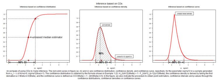
See Figure 1 from Xie and Singh (2011) for a graphical illustration of the CD inference.