Fisher transformation

Definition

Given a set of N bivariate sample pairs (X_i, Y_i), i = 1, ..., N, the sample correlation coefficient r is given by

Here cov ⁡ ( X , Y ) stands for the covariance between the variables X and Y and σ stands for the standard deviation of the respective variable. Fisher's z-transformation of r is defined as

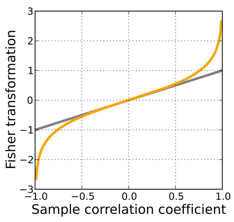
where "ln" is the natural logarithm function and "arctanh" is the inverse hyperbolic tangent function.

If (X, Y) has a bivariate normal distribution with correlation ρ and the pairs (X_i, Y_i) are independent and identically distributed, then z is approximately normally distributed with mean

and standard error

where N is the sample size, and ρ is the true correlation coefficient.

This transformation, and its inverse

can be used to construct a large-sample confidence interval for r using standard normal theory and derivations.

Discussion

The Fisher transformation is an approximate variance-stabilizing transformation for r when X and Y follow a bivariate normal distribution. This means that the variance of z is approximately constant for all values of the population correlation coefficient ρ. Without the Fisher transformation, the variance of r grows smaller as |ρ| gets closer to 1. Since the Fisher transformation is approximately the identity function when |r| < 1/2, it is sometimes useful to remember that the variance of r is well approximated by 1/N as long as |ρ| is not too large and N is not too small. This is related to the fact that the asymptotic variance of r is 1 for bivariate normal data.

The behavior of this transform has been extensively studied since Fisher introduced it in 1915. Fisher himself found the exact distribution of z for data from a bivariate normal distribution in 1921; Gayen in 1951 determined the exact distribution of z for data from a bivariate Type A Edgeworth distribution. Hotelling in 1953 calculated the Taylor series expressions for the moments of z and several related statistics and Hawkins in 1989 discovered the asymptotic distribution of z for data from a distribution with bounded fourth moments.

Other uses

While the Fisher transformation is mainly associated with the Pearson product-moment correlation coefficient for bivariate normal observations, it can also be applied to Spearman's rank correlation coefficient in more general cases. A similar result for the asymptotic distribution applies, but with a minor adjustment factor: see the latter article for details.