Comb filter - Alchetron, The Free Social Encyclopedia

In signal processing, a comb filter adds a delayed version of a signal to itself, causing constructive and destructive interference. The frequency response of a comb filter consists of a series of regularly spaced notches, giving the appearance of a comb.

Applications

Comb filters are used in a variety of signal processing applications. These include:

Cascaded integrator–comb (CIC) filters, commonly used for anti-aliasing during interpolation and decimation operations that change the sample rate of a discrete-time system.

2D and 3D comb filters implemented in hardware (and occasionally software) for PAL and NTSC television decoders. The filters work to reduce artifacts such as dot crawl.

Audio effects, including echo, flanging, and digital waveguide synthesis. For instance, if the delay is set to a few milliseconds, a comb filter can be used to model the effect of acoustic standing waves in a cylindrical cavity or in a vibrating string.

In astronomy the astro-comb promises to increase the precision of existing spectrographs by nearly a hundredfold.

In acoustics, comb filtering can arise in some unwanted ways. For instance, when two loudspeakers are playing the same signal at different distances from the listener, there is a comb filtering effect on the signal. In any enclosed space, listeners hear a mixture of direct sound and reflected sound. Because the reflected sound takes a longer path, it constitutes a delayed version of the direct sound and a comb filter is created where the two combine at the listener.

Technical discussion

Comb filters exist in two different forms, feedforward and feedback; the names refer to the direction in which signals are delayed before they are added to the input.

Comb filters may be implemented in discrete time or continuous time; this article will focus on discrete-time implementations; the properties of the continuous-time comb filter are very similar.

Feedforward form

The general structure of a feedforward comb filter is shown on the right. It may be described by the following difference equation:

y [ n ] = x [ n ] + α x [ n − K ]

where K is the delay length (measured in samples), and α is a scaling factor applied to the delayed signal. If we take the Z transform of both sides of the equation, we obtain:

Y ( z ) = ( 1 + α z − K ) X ( z )

We define the transfer function as:

H ( z ) = Y ( z ) X ( z ) = 1 + α z − K = z K + α z K

Frequency response

To obtain the frequency response of a discrete-time system expressed in the Z domain, we make the substitution z = e j Ω . Therefore, for our feedforward comb filter, we get:

H ( e j Ω ) = 1 + α e − j Ω K

Using Euler's formula, we find that the frequency response is also given by

H ( e j Ω ) = [ 1 + α cos ⁡ ( Ω K ) ] − j α sin ⁡ ( Ω K )

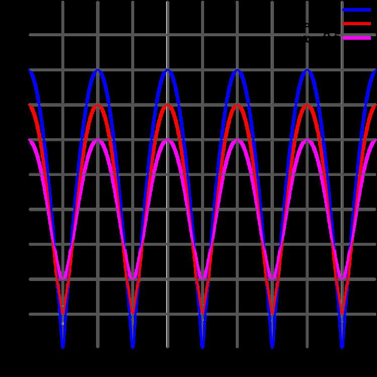
Often of interest is the magnitude response, which ignores phase. This is defined as:

| H ( e j Ω ) | = ℜ { H ( e j Ω ) } 2 + ℑ { H ( e j Ω ) } 2

In the case of the feedforward comb filter, this is:

| H ( e j Ω ) | = ( 1 + α 2 ) + 2 α cos ⁡ ( Ω K )

Notice that the ( 1 + α 2 ) term is constant, whereas the 2 α cos ⁡ ( Ω K ) term varies periodically. Hence the magnitude response of the comb filter is periodic.

The graphs to the right show the magnitude response for various values of α , demonstrating this periodicity. Some important properties:

The response periodically drops to a local minimum (sometimes known as a notch), and periodically rises to a local maximum (sometimes known as a peak).

For positive values of α , the first minimum occurs at half the delay period and repeat at even multiples of the delay frequency thereafter: f = 1 2 K , 3 2 K , 5 2 K . . . .

The levels of the maxima and minima are always equidistant from 1.

When α = ± 1 , the minima have zero amplitude. In this case, the minima are sometimes known as nulls.

The maxima for positive values of α coincide with the minima for negative values of α , and vice versa.

Impulse response

The feedforward comb filter is one of the simplest finite impulse response filters. Its response is simply the initial impulse with a second impulse after the delay.

Pole–zero interpretation

Looking again at the Z-domain transfer function of the feedforward comb filter:

H ( z ) = z K + α z K

we see that the numerator is equal to zero whenever z K = − α . This has K solutions, equally spaced around a circle in the complex plane; these are the zeros of the transfer function. The denominator is zero at z K = 0 , giving K poles at z = 0 . This leads to a pole–zero plot like the ones shown below.

Feedback form

Similarly, the general structure of a feedback comb filter is shown on the right. It may be described by the following difference equation:

y [ n ] = x [ n ] + α y [ n − K ]

If we rearrange this equation so that all terms in y are on the left-hand side, and then take the Z transform, we obtain:

( 1 − α z − K ) Y ( z ) = X ( z )

The transfer function is therefore:

H ( z ) = Y ( z ) X ( z ) = 1 1 − α z − K = z K z K − α

Frequency response

If we make the substitution z = e j Ω into the Z-domain expression for the feedback comb filter, we get:

H ( e j Ω ) = 1 1 − α e − j Ω K

The magnitude response is as follows:

| H ( e j Ω ) | = 1 ( 1 + α 2 ) − 2 α cos ⁡ ( Ω K )

Again, the response is periodic, as the graphs to the right demonstrate. The feedback comb filter has some properties in common with the feedforward form:

The response periodically drops to a local minimum and rises to a local maximum.

The maxima for positive values of α coincide with the minima for negative values of α , and vice versa.

For positive values of α , the first minimum occurs at 0 and repeats at even multiples of the delay frequency thereafter: f = 0 , 1 K , 2 K . . . .

However, there are also some important differences because the magnitude response has a term in the denominator:

The levels of the maxima and minima are no longer equidistant from 1. The maxima have an amplitude of 1 1 − α .

The filter is only stable if | α | is strictly less than 1. As can be seen from the graphs, as | α | increases, the amplitude of the maxima rises increasingly rapidly.

Impulse response

The feedback comb filter is a simple type of infinite impulse response filter. If stable, the response simply consists of a repeating series of impulses decreasing in amplitude over time.

Pole–zero interpretation

Looking again at the Z-domain transfer function of the feedback comb filter:

H ( z ) = z K z K − α

This time, the numerator is zero at z K = 0 , giving K zeros at z = 0 . The denominator is equal to zero whenever z K = α . This has K solutions, equally spaced around a circle in the complex plane; these are the poles of the transfer function. This leads to a pole–zero plot like the ones shown below.

Continuous-time comb filters

Comb filters may also be implemented in continuous time. The feedforward form may be described by the following equation:

y ( t ) = x ( t ) + α x ( t − τ )

where τ is the delay (measured in seconds). This has the following transfer function:

H ( s ) = 1 + α e − s τ

The feedforward form consists of an infinite number of zeros spaced along the jω axis.

The feedback form has the equation:

y ( t ) = x ( t ) + α y ( t − τ )

and the following transfer function:

H ( s ) = 1 1 − α e − s τ

The feedback form consists of an infinite number of poles spaced along the jω axis.

Continuous-time implementations share all the properties of the respective discrete-time implementations.

References

Comb filter Wikipedia

(Text) CC BY-SA

Contents

Applications

Technical discussion

Feedforward form

Frequency response

Impulse response

Pole–zero interpretation

Feedback form

Frequency response

Impulse response

Pole–zero interpretation

Continuous-time comb filters

References