
 | ||
In mathematics, signal processing and control theory, a pole–zero plot is a graphical representation of a rational transfer function in the complex plane which helps to convey certain properties of the system such as:
Contents
A pole-zero plot shows the location in the complex plane of the poles and zeros of the transfer function of a dynamic system, such as a controller, compensator, sensor, equalizer, filter, or communications channel. By convention, the poles of the system are indicated in the plot by an X while the zeroes are indicated by a circle or O.
A pole-zero plot can represent either a continuous-time (CT) or a discrete-time (DT) system. For a CT system, the plane in which the poles and zeros appear is the s plane of the Laplace transform. In this context, the parameter s represents the complex angular frequency, which is the domain of the CT transfer function. For a DT system, the plane is the z plane, where z represents the domain of the Z-transform.
Continuous-time systems
In general, a rational transfer function for a continuous-time LTI system has the form:
where
Either M or N or both may be zero, but in real systems, it should be the case that
Poles and zeros
Region of convergence
The region of convergence (ROC) for a given CT transfer function is a half-plane or vertical strip, either of which contains no poles. In general, the ROC is not unique, and the particular ROC in any given case depends on whether the system is causal or anti-causal.
The ROC is usually chosen to include the imaginary axis since it is important for most practical systems to have BIBO stability.
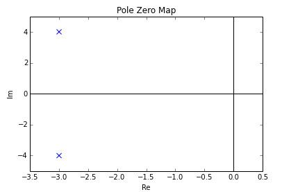
Example
This system has no (finite) zeros and two poles:
and
The pole-zero plot would be:
Notice that these two poles are complex conjugates, which is the necessary and sufficient condition to have real-valued coefficients in the differential equation representing the system.
Discrete-time systems
In general, a rational transfer function for a discrete-time LTI system has the form:
where
Either M or N or both may be zero.
Poles and zeros
Region of convergence
The region of convergence (ROC) for a given DT transfer function is a disk or annulus which contains no poles. In general, the ROC is not unique, and the particular ROC in any given case depends on whether the system is causal or anti-causal.
The ROC is usually chosen to include the unit circle since it is important for most practical systems to have BIBO stability.
Example
If
The only (finite) zero is located at:
The pole–zero plot would be: