Classical control theory - Alchetron, the free social encyclopedia

Classical control theory is a branch of control theory that deals with the behavior of dynamical systems with inputs, and how their behavior is modified by feedback, using the Laplace transform as a basic tool to model such systems.

The usual objective of control theory is to control a system, often called the plant, so its output follows a desired control signal, called the reference, which may be a fixed or changing value. To do this a controller is designed, which monitors the output and compares it with the reference. The difference between actual and desired output, called the error signal, is applied as feedback to the input of the system, to bring the actual output closer to the reference.

Classical control theory deals with linear time-invariant single-input single-output systems. The Laplace transform of the input and output signal of such systems can be calculated. The transfer function relates the Laplace transform of the input and the output.

Feedback

To overcome the limitations of the open-loop controller, classical control theory introduces feedback. A closed-loop controller uses feedback to control states or outputs of a dynamical system. Its name comes from the information path in the system: process inputs (e.g., voltage applied to an electric motor) have an effect on the process outputs (e.g., speed or torque of the motor), which is measured with sensors and processed by the controller; the result (the control signal) is "fed back" as input to the process, closing the loop.

Closed-loop controllers have the following advantages over open-loop controllers:

disturbance rejection (such as hills in the cruise control example above)

guaranteed performance even with model uncertainties, when the model structure does not match perfectly the real process and the model parameters are not exact

unstable processes can be stabilized

reduced sensitivity to parameter variations

improved reference tracking performance

In some systems, closed-loop and open-loop control are used simultaneously. In such systems, the open-loop control is termed feedforward and serves to further improve reference tracking performance.

A common closed-loop controller architecture is the PID controller.

Classical vs modern

A Physical system can be modeled in the "time domain", where the response of a given system is a function of the various inputs, the previous system values, and time. As time progresses, the state of the system and its response change. However, time-domain models for systems are frequently modeled using high-order differential equations which can become impossibly difficult for humans to solve and some of which can even become impossible for modern computer systems to solve efficiently.

To counteract this problem, classical control theory uses the Laplace transform to change an Ordinary Differential Equation (ODE) in the time domain into a regular algebraic polynomial in the transform domain. Once a given system has been converted into the transform domain it can be manipulated with greater ease.

Modern control theory, instead of changing domains to avoid the complexities of time-domain ODE mathematics, converts the differential equations into a system of lower-order time domain equations called state equations, which can then be manipulated using techniques from linear algebra.

Laplace transform

Classical control theory uses the Laplace transform to model the systems and signals. The Laplace transform is a frequency-domain approach for continuous time signals irrespective of whether the system is stable or unstable. The Laplace transform of a function f(t), defined for all real numbers t ≥ 0, is the function F(s), which is a unilateral transform defined by

F ( s ) = ∫ 0 ∞ e − s t f ( t ) d t

where s is a complex number frequency parameter

s = σ + i ω , with real numbers σ and ω.

Closed-loop transfer function

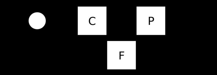
The output of the system y(t) is fed back through a sensor measurement F to the reference value r(t). The controller C then takes the error e (difference) between the reference and the output to change the inputs u to the system under control P. This is shown in the figure. This kind of controller is a closed-loop controller or feedback controller.

This is called a single-input-single-output (SISO) control system; MIMO (i.e., Multi-Input-Multi-Output) systems, with more than one input/output, are common. In such cases variables are represented through vectors instead of simple scalar values. For some distributed parameter systems the vectors may be infinite-dimensional (typically functions).

If we assume the controller C, the plant P, and the sensor F are linear and time-invariant (i.e., elements of their transfer function C(s), P(s), and F(s) do not depend on time), the systems above can be analysed using the Laplace transform on the variables. This gives the following relations:

Y ( s ) = P ( s ) U ( s ) U ( s ) = C ( s ) E ( s ) E ( s ) = R ( s ) − F ( s ) Y ( s ) .

Solving for Y(s) in terms of R(s) gives

Y ( s ) = ( P ( s ) C ( s ) 1 + F ( s ) P ( s ) C ( s ) ) R ( s ) = H ( s ) R ( s ) .

The expression H ( s ) = P ( s ) C ( s ) 1 + F ( s ) P ( s ) C ( s ) is referred to as the closed-loop transfer function of the system. The numerator is the forward (open-loop) gain from r to y, and the denominator is one plus the gain in going around the feedback loop, the so-called loop gain. If | P ( s ) C ( s ) | ≫ 1 , i.e., it has a large norm with each value of s, and if | F ( s ) | ≈ 1 , then Y(s) is approximately equal to R(s) and the output closely tracks the reference input.

PID controller

The PID controller is probably the most-used feedback control design. PID is an initialism for Proportional-Integral-Derivative, referring to the three terms operating on the error signal to produce a control signal. If u(t) is the control signal sent to the system, y(t) is the measured output and r(t) is the desired output, and tracking error e ( t ) = r ( t ) − y ( t ) , a PID controller has the general form

u ( t ) = K P e ( t ) + K I ∫ e ( t ) d t + K D d d t e ( t ) .

The desired closed loop dynamics is obtained by adjusting the three parameters K P , K I and K D , often iteratively by "tuning" and without specific knowledge of a plant model. Stability can often be ensured using only the proportional term. The integral term permits the rejection of a step disturbance (often a striking specification in process control). The derivative term is used to provide damping or shaping of the response. PID controllers are the most well established class of control systems: however, they cannot be used in several more complicated cases, especially if multiple-input multiple-output systems (MIMO) systems are considered.

Applying Laplace transformation results in the transformed PID controller equation

u ( s ) = K P e ( s ) + K I 1 s e ( s ) + K D s e ( s ) u ( s ) = ( K P + K I 1 s + K D s ) e ( s )

with the PID controller transfer function

C ( s ) = ( K P + K I 1 s + K D s ) .

There exists a nice example of the closed-loop system discussed above. If we take

PID controller transfer function in series form

C ( s ) = K ( 1 + 1 s T i ) ( 1 + s T d )

1st order filter in feedback loop

F ( s ) = 1 1 + s T f

linear actuator with filtered input

P ( s ) = A 1 + s T p , A = const

and insert all this into expression for closed-loop transfer function H(s), then tuning is very easy: simply put

K = 1 A , T i = T f , T d = T p

and get H(s) = 1 identically.

For practical PID controllers, a pure differentiator is neither physically realisable nor desirable due to amplification of noise and resonant modes in the system. Therefore, a phase-lead compensator type approach is used instead, or a differentiator with low-pass roll-off.

Tools

Classical control theory uses an array of tools to analyze systems and design controllers for such systems. Tools include the root locus, the Nyquist stability criterion, the Bode plot, the gain margin and phase margin.

References

Classical control theory Wikipedia

(Text) CC BY-SA

Contents