Center manifold - Alchetron, The Free Social Encyclopedia

In mathematics, the center manifold of an equilibrium point of a dynamical system consists of orbits whose behavior around the equilibrium point is not controlled by either the attraction of the stable manifold or the repulsion of the unstable manifold. The first step when studying equilibrium points of dynamical systems is to linearize the system. The eigenvectors corresponding to eigenvalues with negative real part form the stable eigenspace, which gives rise to the stable manifold. Similarly, eigenvalues with positive real part yield the unstable manifold.

This concludes the story if the equilibrium point is hyperbolic (i.e., all eigenvalues of the linearization have nonzero real part). However, if there are eigenvalues whose real part is zero, then these give rise to the center manifold. If the eigenvalues are precisely zero, rather than just real part being zero, then these more specifically give rise to a slow manifold. The behavior on the center (slow) manifold is generally not determined by the linearization and thus is more difficult to study.

Center manifolds play an important role in: bifurcation theory because interesting behavior takes place on the center manifold; and multiscale mathematics because the long time dynamics often are attracted to a relatively simple center manifold.

Definition

Let d x d t = f ( x ) be a dynamical system with equilibrium point x ∗ . The linearization of the system near the equilibrium point is

d x d t = A x , where Jacobian A = d f d x ( x ∗ ) .

The matrix A defines three main subspaces:

the stable subspace, which is spanned by the generalized eigenvectors corresponding to the eigenvalues λ with Re ⁡ λ < 0 ;

the unstable subspace, which is spanned by the generalized eigenvectors corresponding to the eigenvalues λ with Re ⁡ λ > 0 ;

the center subspace, which is spanned by the generalized eigenvectors corresponding to the eigenvalues λ with Re ⁡ λ = 0 .

Depending upon the application, other subspaces of interest include center-stable, center-unstable, sub-center, slow, and fast subspaces. These subspaces are all invariant subspaces of the linearized equation.

Corresponding to the linearized system, the nonlinear system has invariant manifolds, each consisting of sets of orbits of the nonlinear system.

An invariant manifold tangent to the stable subspace and with the same dimension is the stable manifold.

The unstable manifold is of the same dimension and tangent to the unstable subspace.

A center manifold is of the same dimension and tangent to the center subspace. If, as is common, the eigenvalues of the center subspace are all precisely zero, rather than just real part zero, then a center manifold is often called a slow manifold.

Center manifold theorems

The center manifold existence theorem states that if the right-hand side function f ( x ) is C r ( r times continuously differentiable), then at every equilibrium point there exists a neighborhood of some finite size in which there is at least one of

a unique C r stable manifold,

a unique C r unstable manifold,

and a (not necessarily unique) C r − 1 center manifold.

In example applications, a nonlinear coordinate transform to a normal form can clearly separate these three manifolds. A web service [1] currently undertakes the necessary computer algebra for a range of finite-dimensional systems.

In the case when the unstable manifold does not exist, center manifolds are often relevant to modelling. The center manifold emergence theorem then says that the neighborhood may be chosen so that all solutions of the system staying in the neighborhood tend exponentially quickly to some solution y ( t ) on the center manifold. That is, x ( t ) = y ( t ) + O ( e − β ′ t ) as t → ∞ , for some rate β ′ . This theorem asserts that for a wide variety of initial conditions the solutions of the full system decay exponentially quickly to a solution on the relatively low dimensional center manifold.

A third theorem, the approximation theorem, asserts that if an approximate expression for such invariant manifolds, say x = X ( s ) , satisfies the differential equation for the system to residuals O ( | s | p ) as s → 0 , then the invariant manifold is approximated by x = X ( s ) to an error of the same order, namely O ( | s | p ) .

However, some applications, such as to shear dispersion, require an infinite-dimensional center manifold. The most general and powerful theory was developed by Aulbach and Wanner They addressed non-autonomous dynamical systems d x d t = f ( x , t ) in infinite dimensions, with potentially infinite dimensional stable, unstable and center manifolds. Further, they usefully generalised the definition of the manifolds so that the center manifold is associated with eigenvalues such that | Re ⁡ λ | ≤ α , the stable manifold with eigenvalues Re ⁡ λ ≤ − β < − r α , and unstable manifold with eigenvalues Re ⁡ λ ≥ β > r α . They proved existence of these manifolds, and the emergence of a center manifold, via nonlinear coordinate transforms. Potzsche and Rasmussen established a corresponding approximation theorem for such infinite dimensional, non-autonomous systems.

Center manifold and the analysis of nonlinear systems

As the stability of the equilibrium correlates with the "stability" of its manifolds, the existence of a center manifold brings up the question about the dynamics on the center manifold. This is analyzed by the center manifold reduction, which, in combination with some system parameter μ, leads to the concepts of bifurcations.

Correspondingly, two web services currently undertake the necessary computer algebra to construct just the center manifold for a wide range of finite-dimensional systems (provided they are in multinomial form).

One web service [2] constructs slow manifolds for systems which are linearly diagonalised, but which may be non-autonomous or stochastic.

Another web service [3] constructs center manifolds for systems with general linearisation, but only for autonomous systems.

Examples

The Wikipedia entry on slow manifolds gives more examples.

A simple example

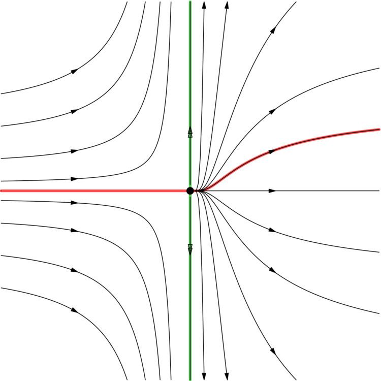
Consider the system

x ˙ = x 2 , y ˙ = y .

The unstable manifold at the origin is the y axis, and the stable manifold is the trivial set {(0, 0)}. Any orbit not on the stable manifold satisfies an equation on the form y = A e − 1 / x for some real constant A. It follows that for any real A, we can create a center manifold by piecing together the curve y = A e − 1 / x for x > 0 with the negative x axis (including the origin). Moreover, all center manifolds have this potential non-uniqueness, although often the non-uniqueness only occurs in unphysical complex values of the variables.

Delay differential equations often have Hopf bifurcations

Another example shows how a center manifold models the Hopf bifurcation that occurs for parameter a ≈ 4 in the delay differential equation d x / d t = − a x ( t − 1 ) − 2 x 2 − x 3 . Strictly, the delay makes this DE infinite-dimensional.

Fortunately, we may approximate such delays by the following trick that keeps the dimensionality finite. Define u 1 ( t ) = x ( t ) and approximate the time delayed variable, x ( t − 1 ) ≈ u 3 ( t ) , by using the intermediaries d u 2 / d t = 2 ( u 1 − u 2 ) and d u 3 / d t = 2 ( u 2 − u 3 ) .

For parameter near critical, a = 4 + α , the delay differential equation is then approximated by the system

d u d t = [ 0 0 − 4 2 − 2 0 0 2 − 2 ] u + [ − α u 3 − 2 u 1 2 − u 1 3 0 0 ] .

Copying and pasting the appropriate entries, the web service [4] finds that in terms of a complex amplitude s ( t ) and its complex conjugate s ¯ ( t ) , the center manifold

u = [ e i 2 t s + e − i 2 t s ¯ 1 − i 2 e i 2 t s + 1 + i 2 e − i 2 t s ¯ − i 2 e i 2 t s + i 2 e − i 2 t s ¯ ] + O ( α + | s | 2 )

and the evolution on the center manifold is

d s d t = [ 1 + 2 i 10 α s − 3 + 16 i 15 | s | 2 s ] + O ( α 2 + | s | 4 )

This evolution shows the origin is linearly unstable for α > 0 ( a > 4 ) , but the cubic nonlinearity then stabilises nearby limit cycles as in classic Hopf bifurcation.

References

Center manifold Wikipedia

(Text) CC BY-SA

Contents