Capillary bridges

History

Capillary bridges have been studied for over 200 years. The question was raised for the first time by Josef Louis Lagrange in 1760, and interest was further spread by the French astronomer and mathematician C. Delaunay. Delaunay found an entirely new class of axially symmetrical surfaces of constant mean curvature. The formulation and the proof of his theorem had a long story. It began with Euler's proposition of new figure, called cathenoid. (Much later, Kenmotsu solved the complex nonlinear equations, describing this class of surfaces. However, his solution is of little practical importance because it has no geometrical interpretation.) J. Plateau showed the existence of such shapes with given boundaries. The problem was named after him Plateau's problem.
Many scientists contributed to the solution of the problem. One of them is Thomas Young. Pierre Simon Laplace contributed the notion of capillary tension. Laplace even formulated the widely known nowadays condition for mechanical equilibrium between two fluids, divided by a capillary surface P_γ=ΔP i.e. capillary pressure between two phases is balanced by their adjacent pressure difference.
A general survey on capillary bridge behavior in gravity field is completed by Myshkis and Babskii.
In the last century a lot of efforts were put of study of surface forces that drive capillary effects of bridging. There was established that these forces result from intermolecular forces and become significant in thin fluid gaps (<10 nm) between two surfaces.
The instability of capillary bridges was discussed in first time by Rayleigh. He demonstrated that a liquid jet or capillary cylindrical surface became unstable when the ratio between its length, H to the radius R, becomes bigger than 2π. In these conditions of small sinusoidal perturbations with wavelength bigger than it perimeter, the cylinder surface area becomes larger than the one of unperturbed cylinder with the same volume and thus it becomes unstable. Later, Hove formulated the variational requirements for the stability of axisymmetric capillary surfaces (unbounded) in absence of gravity and with disturbances constarined to constant volume. He first solved Young-Laplace equation for equilibrium shapes and showed that the Legendre condition for the second variation is always satisfied. Therefore the stability is determined by the absence of negative eigenvalue of the linearized Young-Laplace equation. This approach of determining stability from second variation is used now widely. Pertirbation methods became very successful despite that nonlinear nature of capillary interaction can limit their application. Other methods now include direct simulation. To that moment most methods for stability determination required calculation of equilibrium as a basis for perturbations. There appeared a new idea that stability may be deduced from equilibrium states. The proposition was further proven by Pitts for axisymmetric constant volume. In the following years Vogel extended the theory. He examined the case of axisymmetric capillary bridges with constant volumes and the stability changes correspond to turning points. The recent development of bifurcation theory proved that exchange of stability between turning points and branch points is a general phenomenon.

Applications and Occurrences

Recent studies indicated that ancient Egyptians used the properties of sand to create capillary bridges by using water on it. In this way, they reduced surface friction and were capable to move statues and heavy pyramid stones. Some contemporary arts, like Sand art, are also close related to capability of water to bridge particles. In Atomic force microscopy, when one works in higher humidity environment, his studies might be affected by the appearance of nanosized capillary bridges. These bridges appear when the working tip approaches the studied sample. Capillary bridges also play important role in soldering process.

Capillary bridges also widely spread in living nature. Bugs, flies, grasshoppers and tree frogs are capable to adhere to vertical rough surfaces because of their ability to inject wetting liquid into the pad-substrate contact area. This way is created long range attractive interaction due to the formation of capillary bridges. Many medical problems involving respiratory diseases, and the health of the body joints depend on tiny capillary bridges. Liquid bridges are now commonly used in growth of cell cultures because of the need to mimic work of living tissues in scientific research.

General equations

General solution for the profile of capillary is known from consideration of unduloid or nodoid curvature
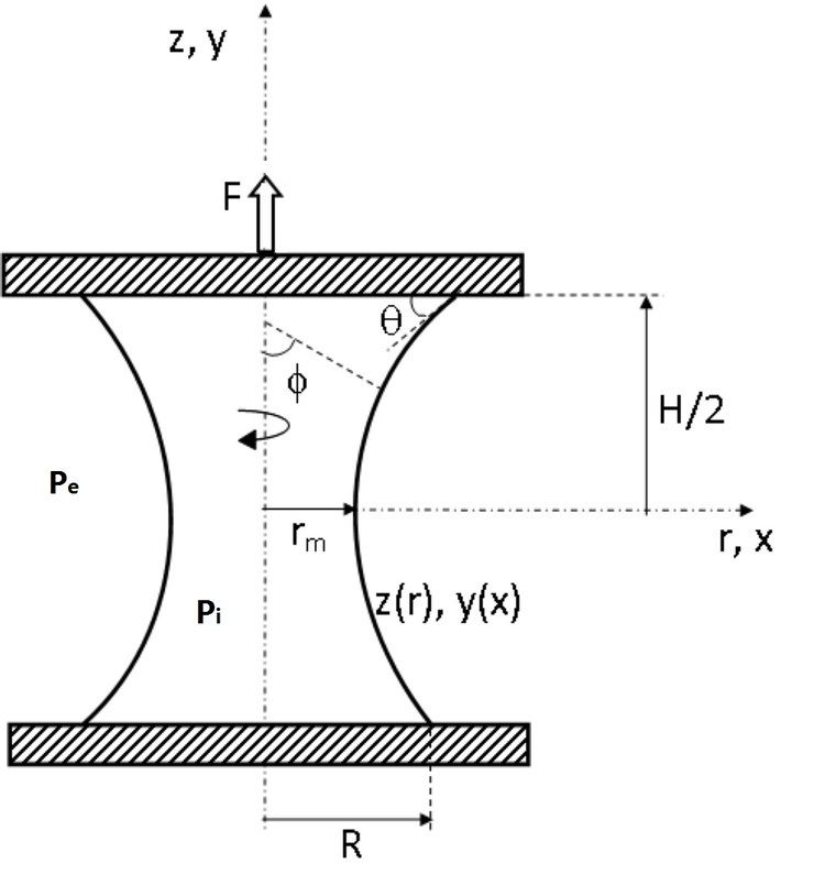
Let's assume the following cylindrical coordinate system: z shows axis of revolution; r represents radii of curvature and φ is the angle between the normal and the positive z axis. The nodoid has vertical tangents at r = r₁ and r = r₂ and horizontal tangent at r = r₃. When the φ is the angle between the normal to the interface and positive z axis then φ is equal to 90°, 0°, -90° for nodoid. This way the Young-Laplace equation may be written with account of total curvature:

where R₁, R₂ are the radii of curvature and γ is interfacial surface tension.
The integration of the equation is called The first integral and for nodoid with the boundary conditions mentioned above yields:

Since:

One finds:

After the integration, the obtained equation is called The second integral:

where: F and E are elliptic integrals of first and second kind, k 2 = r 2 2 − r 1 2 r 2 2 and φ is related to r according to: sin 2 ⁡ ϕ = r 2 2 − r 2 r 2 2 − r 1 2 .
The unduloid has only vertical tangents at r=r₁ and r=r₂, where φ = + 90. In a completely analogous way:

The second integral for unduloid is obtained:

Where the relation between parameters k and φ are defined the same way as above. In the limiting case r₁=0, both nodoid and unduloid consist of a series of spheres. When r₁=r₂. The last and the very interesting limiting case is catenoid. The Laplace equation is reduced to:

It integration can be represented in very convenient form, in cylindrical coordinate system, called catenary equation:

Equation (9) is important because it shows in some simplification all issues, related to the capillary bridges, transparent. Drawing in dimensionless coordinates exhibit a maximum, that distinguishes two branches. One of them is energetically favorable and come up to existence in statics while the other (in dashed line) is not energetically favorable. Maximum is important because when stretching quasi-equilibrium way capillary bridge, if maximum is reached, it breakage takes place. Catenoids with energetically unfavorable dimensions may form during process of dynamical stretching/pressing. Zero capillary pressure C=0 is natural for classical catenoid (capillary soap surface stretched between two coaxial rings). When typical capillary bridge comes to catenoidal state of C = 0, despite that it surface properties are the same as classical cathenoid, it is more appropriate to be presented as scaled by cube root of its volume rather than the radius, R.
It is important to note that all described curves are found by rolling a conic section without slip along z axis. The unduloid is described by the focus of rolling ellipse, which can degenerate into a line, a sphere or a parabola, leading to the corresponding limiting cases. Similarly, a nodoid is described by the focus of a rolling hyperbola.

Statics of Capillary Bridge between Two Flat Surfaces

The mechanical equilibrium comprises the pressure balance on liquid/gas interface and the external force on plates, ΔP, balancing the capillary attraction or repulsion, P_y, i.e.ΔP = P_y . Upon neglecting gravity effects and other external fields, the pressure balance is ΔP=P_i - P_e (The indexes "i" and "e" denote correspondingly internal and external pressures). In case of axial symmetry, the equation for capillary pressure takes the form:

,

where γ is interfacial liquid/gas tension; r is radial coordinate and φ is the angle between the axis symmetry and normal to interface generatrix.
The first integral is easily obtained regarding dimensionless capillary pressure at the contact with surface:

. where C = P y r m 2 γ , dimensionless radius at the contact is X = R r m and θ is the contact angle. The relation shows that capillary pressure can be positive or negative. The shape of capillary bridges is governed by the equation:

where the equation is obtained after substitution sin ⁡ ϕ = d y d x cos ⁡ ϕ is made in Eq. (11) and scalling x = r r m is introduced.

Thin liquid bridge

In contrast to cases with increasing height of capillary bridges, that poses variety of profile shapes, the flattening (thinning) toward zero thickness has much more universal character. The universality appears when H<<R (fig. 1). Equation (11) may be written:

The generatrix converges to equation:

Uppon integration, the equation yields:

The dimensionless circular radii 1/2C coincides with capillary bridge radii of curvature. The positive sign '+' represents generatrix profile of concave bridge and negative '-', oblate.

Definition domain of liquid capillary bridges

The observations, presented in fig. 5 indicate that a domain of capillary bridges existence can be defined. Therefore, if stretching of a liquid bridge it might discontinue its existence not only because of raising instabilities but also because of reaching of some points that the shape can not exist anymore. The estimation of definition domain requires manipulation of integrated equations for capillary bridge height and its volume. Both they are integrable but the integrals are improper. The applied method includes splitting of the integrals on two parts: singular but integrable analytically and regular but integrable only numerical way.
After the integration, for the capillary bridge height is obtained
:

Similar way for contact radius R, is obtained the integrated equation
:

Where γ ( C ) = [ 1 − ( 1 − 2 C ) 2 C 2 ] and α ( C , X ) = 1 2 C arcsin ⁡ [ γ ( C ) − X 2 2 C 2 1 − 2 C ]

In fig. 6 are shown number of stable static states of liquid capillary bridge, represented by two characteristic parameters: (i) dimensionless height that is obtained by scaling of capillary bridge height by cubic root of its volume Eq. (16) and (ii) its radius, also scaled by cubic root of volume, Eq. (17). The partially analytical solutions, obtained for these two parameters, are presented above. The solutions somehow differs from widely accepted Plateau's approach [by elliptical functions, Eq. (7)], because they offer convenient numerical approach for integration of regular integrals, while irregular part of the equation was integrated analytically.

Concave capillary bridge

The case of concave capillary bridge is presented by isogones for contact angles below π 2 in fig. 6, ( 0 ≤ θ < π 2 ). The isogones show well defined maximum d H ∗ d R ∗ ≡ d H d R = 0 . This maximum is noted by dot for each isogone. It again, similarly to a simple catenoid, separates two branches. The left branch is energetically favourable while the right one is energetically unfavourable.

Cylindrical capillary bridge

This case is analysed well by Rayleigh. Note that the definition domain in his case shows no limitations and it goes to infinity, fig. 6, ( θ = π 2 ). However, the breakage of cylindrical capillary bridges is usually observed. It takes place as result from well studied instability known now as Rayleigh instability. The definition domain for 90° isogone in shown in fig 6 by dashed line.

Convex capillary bridge

The case of convex capillary bridges is presented in fig. 6, ( π 2 < θ ≤ π ) left from the domain of cylindrical case.

Stability of Capillary Bridge between Two Flat Surfaces

Equilibrium shapes and stability limits for capillary liquid bridges are subject to many theoretical and experimental studies. Studies are mostly concentrated on investigation of bridges between equals disks under gravitational conditions. It is well known that for each value of Bond number B o = ρ g R 2 γ (where: g is Earth gravity, γ is the surface tension and R is radius of the contact) the stability diagramm can be represented by a single closed piecewise curve on the slenderness/dimensionless volume plane. Slenderness is defined as H 2 R , and the dimensionless volume is capillary bridge volume divided on cylinder volume with the same height, H and radius R: V π R 2 H .

If both slenderness and liquid volume are small enough, the stability limits are governed by detachment of liquid shape from the edges of the disks (three-phase contact line), AB line in fig. 7. The line BC represents minimum in volume that corresponds to axisymmetrical breakage. It is known in literature as minimum volume stability limit. The curve CA represents another limit to stability, characterizing maximum volume. It is upper bound to the stability region. There also exists a transition region between minimum and maximum volume stability. It is not yet clearly defined and thus is noted by dashed line in fig. 7.