
 | ||
In fluid dynamics, the Camassa–Holm equation is the integrable, dimensionless and non-linear partial differential equation
Contents
- Relation to waves in shallow water
- Hamiltonian structure
- Integrability
- Exact solutions
- Wave breaking
- Long time asymptotics
- References
The equation was introduced by Camassa and Holm as a bi-Hamiltonian model for waves in shallow water, and in this context the parameter κ is positive and the solitary wave solutions are smooth solitons.
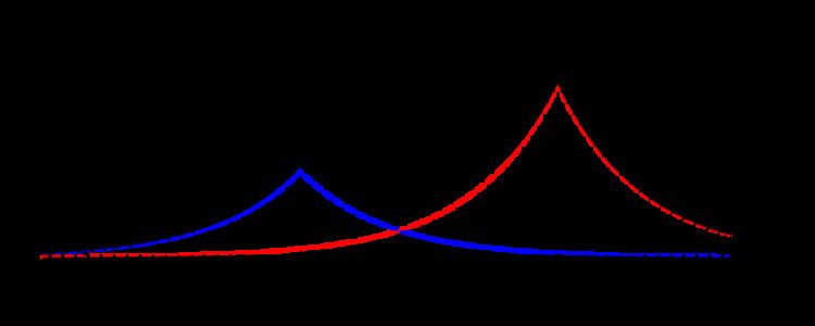
In the special case that κ is equal to zero, the Camassa–Holm equation has peakon solutions: solitons with a sharp peak, so with a discontinuity at the peak in the wave slope.
Relation to waves in shallow water
The Camassa–Holm equation can be written as the system of equations:
with p the (dimensionless) pressure or surface elevation. This shows that the Camassa–Holm equation is a model for shallow water waves with non-hydrostatic pressure and a water layer on a horizontal bed.
The linear dispersion characteristics of the Camassa–Holm equation are:
with ω the angular frequency and k the wavenumber. Not surprisingly, this is of similar form as the one for the Korteweg–de Vries equation, provided κ is non-zero. For κ equal to zero, the Camassa–Holm equation has no frequency dispersion — moreover, the linear phase speed is zero for this case. As a result, κ is the phase speed for the long-wave limit of k approaching zero, and the Camassa–Holm equation is (if κ is non-zero) a model for one-directional wave propagation like the Korteweg–de Vries equation.
Hamiltonian structure
Introducing the momentum m as
then two compatible Hamiltonian descriptions of the Camassa–Holm equation are:
Integrability
The Camassa–Holm equation is an integrable system. Integrability means that there is a change of variables (action-angle variables) such that the evolution equation in the new variables is equivalent to a linear flow at constant speed. This change of variables is achieved by studying an associated isospectral/scattering problem, and is reminiscent of the fact that integrable classical Hamiltonian systems are equivalent to linear flows at constant speed on tori. The Camassa–Holm equation is integrable provided that the momentum
is positive — see and for a detailed description of the spectrum associated to the isospectral problem, for the inverse spectral problem in the case of spatially periodic smooth solutions, and for the inverse scattering approach in the case of smooth solutions that decay at infinity.
Exact solutions
Traveling waves are solutions of the form
representing waves of permanent shape f that propagate at constant speed c. These waves are called solitary waves if they are localized disturbances, that is, if the wave profile f decays at infinity. If the solitary waves retain their shape and speed after interacting with other waves of the same type, we say that the solitary waves are solitons. There is a close connection between integrability and solitons. In the limiting case when κ = 0 the solitons become peaked (shaped like the graph of the function f(x) = e−|x|), and they are then called peakons. It is possible to provide explicit formulas for the peakon interactions, visualizing thus the fact that they are solitons. For the smooth solitons the soliton interactions are less elegant. This is due in part to the fact that, unlike the peakons, the smooth solitons are relatively easy to describe qualitatively — they are smooth, decaying exponentially fast at infinity, symmetric with respect to the crest, and with two inflection points — but explicit formulas are not available. Notice also that the solitary waves are orbitally stable i.e. their shape is stable under small perturbations, both for the smooth solitons and for the peakons.
Wave breaking
The Camassa–Holm equation models breaking waves: a smooth initial profile with sufficient decay at infinity develops into either a wave that exists for all times or into a breaking wave (wave breaking being characterized by the fact that the solution remains bounded but its slope becomes unbounded in finite time). The fact that the equations admits solutions of this type was discovered by Camassa and Holm and these considerations were subsequently put on a firm mathematical basis. It is known that the only way singularities can occur in solutions is in the form of breaking waves. Moreover, from the knowledge of a smooth initial profile it is possible to predict (via a necessary and sufficient condition) whether wave breaking occurs or not. As for the continuation of solutions after wave breaking, two scenarios are possible: the conservative case and the dissipative case (with the first characterized by conservation of the energy, while the dissipative scenario accounts for loss of energy due to breaking).
Long-time asymptotics
It can be shown that for sufficiently fast decaying smooth initial conditions with positive momentum splits into a finite number and solitons plus a decaying dispersive part. More precisely, one can show the following for