CORDIC

History

Similar mathematical techniques were published by Henry Briggs as early as 1624 or Robert Flower in 1771, but CORDIC is optimized for low-complexity finite-state CPUs.

CORDIC was conceived in 1956 by Jack E. Volder at the aeroelectronics department of Convair out of necessity to replace the analog resolver in the B-58 bomber's navigation computer by a more accurate and performant real-time digital solution. Therefore, CORDIC is sometimes referred to as digital resolver.

In his research Volder was inspired by a formula in the 1946 edition of the CRC Handbook of Chemistry and Physics:

His research led to an internal technical report proposing the CORDIC algorithm to solve sine and cosine functions and a prototypical computer implementing it. The report also discussed the possibility to compute hyperbolic coordinate rotation, logarithms and exponential functions with modified CORDIC algorithms. Utilizing CORDIC for multiplication and division was also conceived at this time. Based on the CORDIC principle, Dan H. Daggett, a colleague of Volder at Convair, developed conversion algorithms between binary and binary-coded decimal (BCD).

In 1958, Convair finally started to build a demonstration system to solve radar fix-taking problems named CORDIC I, completed in 1960 without Volder, who had left the company already. More universal CORDIC II models A (stationary) and B (airborne) were built and tested by Daggett and Harry Schuss in 1962.

Volder's CORDIC algorithm was first described in public in 1959, which caused it to be incorporated into navigation computers by companies including Martin-Orlando, Computer Control, Litton, Kearfott, Lear-Siegler, Sperry, Raytheon, and Collins Radio soon.

Volder teamed up with Malcolm MacMillan to build Athena, a fixed-point desktop calculator utilizing his binary CORDIC algorithm. The design was introduced to Hewlett-Packard in June 1965, but not accepted. Still, MacMillan introduced David S. Cochran (HP) to Volder's algorithm and when Cochran later met Volder he referred him to a similar approach John E. Meggitt (IBM) had proposed as pseudo-multiplication and pseudo-division in 1961. Meggitt's method was also suggesting the use of base 10 rather than base 2, as used by Volder's CORDIC so far. These efforts led to the ROMable logic implementation of a decimal CORDIC prototype machine inside of Hewlett-Packard in 1966, build by and conceptually derived from Thomas E. Osborne's prototypical Green Machine, a four-function, floating-point desktop calculator he had completed in DTL logic in December 1964. This project resulted in the public demonstration of Hewlett-Packard's first desktop calculator with scientific functions, the hp 9100A in March 1968, with series production starting later that year.

When Wang Laboratories found that the hp 9100A used an approach similar to the factor combining method in their earlier LOCI-1 (September 1964) and LOCI-2 (January 1965) Logarithmic Computing Instrument desktop calculators, they unsuccessfully accused Hewlett-Packard of infringement of one of An Wang's patents in 1968.

John Stephen Walther at Hewlett-Packard generalized the algorithm into the Unified CORDIC algorithm in 1971, allowing it to calculate hyperbolic and exponential functions, logarithms, multiplications, divisions, and square roots. The CORDIC subroutines for trigonometric and hyperbolic functions could share most of their code. This development resulted in the first scientific handheld calculator, the HP-35 in 1972.

Originally, CORDIC was implemented only using the binary numeral system and despite Meggitt suggesting the use of the decimal system for his pseudo-multiplication approach, decimal CORDIC continued to remain mostly unheard of for several more years, so that Hermann Schmid and Anthony Bogacki still suggested it as a novelty as late as 1973 and it was found only later that Hewlett-Packard had implemented it in 1966 already.

Decimal CORDIC became widely used in pocket calculators, most of which operate in binary-coded decimal (BCD) rather than binary. This change in the input and output format did not alter CORDIC's core calculation algorithms. CORDIC is particularly well-suited for handheld calculators, in which low cost – and thus low chip gate count – is much more important than speed.

CORDIC has been implemented in the Intel 8087, 80287, 80387 up to the 80486 coprocessor series as well as in the Motorola 68881 and 68882 for some kinds of floating-point instructions, mainly as a way to reduce the gate counts (and complexity) of the FPU sub-system.

Applications

CORDIC uses simple shift-add operations for several computing tasks such as the calculation of trigonometric, hyperbolic and logarithmic functions, real and complex multiplications, division, square-root calculation, solution of linear systems, eigenvalue estimation, singular value decomposition, QR factorization and many others. As a consequence, CORDIC has been used for applications in diverse areas such as signal and image processing, communication systems, robotics and 3D graphics apart from general scientific and technical computation.

Hardware

CORDIC is generally faster than other approaches when a hardware multiplier is not available (e.g., a microcontroller), or when the number of gates required to implement the functions it supports should be minimized (e.g., in an FPGA or ASIC).

On the other hand, when a hardware multiplier is available (e.g., in a DSP microprocessor), table-lookup methods and power series are generally faster than CORDIC. In recent years, the CORDIC algorithm has been used extensively for various biomedical applications, especially in FPGA implementations.

Software

Many older systems with integer-only CPUs have implemented CORDIC to varying extents as part of their IEEE floating-point libraries. As most modern general-purpose CPUs have floating-point registers with common operations such as add, subtract, multiply, divide, sine, cosine, square root, log₁₀, natural log, the need to implement CORDIC in them with software is nearly non-existent. Only microcontroller or special safety and time-constrained software applications would need to consider using CORDIC.

Rotation mode

CORDIC can be used to calculate a number of different functions. This explanation shows how to use CORDIC in rotation mode to calculate the sine and cosine of an angle, and assumes the desired angle is given in radians and represented in a fixed-point format. To determine the sine or cosine for an angle β , the y or x coordinate of a point on the unit circle corresponding to the desired angle must be found. Using CORDIC, one would start with the vector v 0 :

In the first iteration, this vector is rotated 45° counterclockwise to get the vector v 1 . Successive iterations rotate the vector in one or the other direction by size-decreasing steps, until the desired angle has been achieved. Step i size is arctan ⁡ ( 2 − i ) for i = 0 , 1 , 2 , . . . .

More formally, every iteration calculates a rotation, which is performed by multiplying the vector v i − 1 with the rotation matrix R i :

The rotation matrix is given by:

Using the following two trigonometric identities:

the rotation matrix becomes:

The expression for the rotated vector v i = R i v i − 1 then becomes:

where x i − 1 and y i − 1 are the components of v i − 1 . Restricting the angles γ i so that tan ⁡ ( γ i ) takes on the values ± 2 − i , the multiplication with the tangent can be replaced by a division by a power of two, which is efficiently done in digital computer hardware using a bit shift. The expression then becomes:

where

and σ i can have the values of −1 or 1, and is used to determine the direction of the rotation; if the angle γ i is positive then σ i is +1, otherwise it is −1.

K i can be ignored in the iterative process and then applied afterward with a scaling factor:

which is calculated in advance and stored in a table, or as a single constant if the number of iterations is fixed. This correction could also be made in advance, by scaling v 0 and hence saving a multiplication. Additionally it can be noted that:

to allow further reduction of the algorithm's complexity. Some applications may avoid correcting for K altogether, resulting in a processing gain A :

After a sufficient number of iterations, the vector's angle will be close to the wanted angle β . For most ordinary purposes, 40 iterations (n = 40) is sufficient to obtain the correct result to the 10th decimal place.

The only task left is to determine if the rotation should be clockwise or counterclockwise at each iteration (choosing the value of σ ). This is done by keeping track of how much the angle was rotated at each iteration and subtracting that from the wanted angle; then in order to get closer to the wanted angle β , if β n + 1 is positive, the rotation is clockwise, otherwise it is negative and the rotation is counterclockwise.

The values of γ n must also be precomputed and stored. But for small angles, arctan ⁡ ( γ n ) = γ n in fixed-point representation, reducing table size.

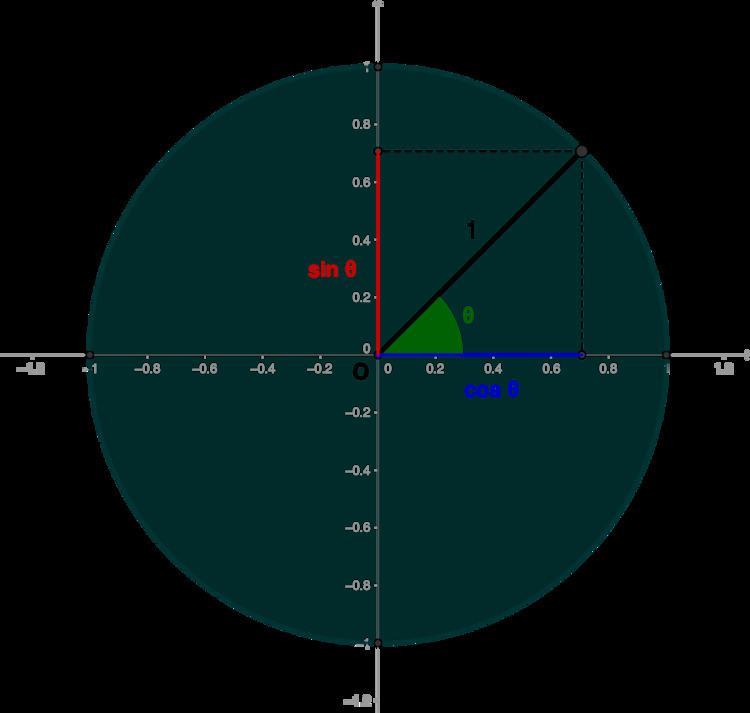
As can be seen in the illustration above, the sine of the angle β is the y coordinate of the final vector v n , while the x coordinate is the cosine value.

Vectoring mode

The rotation-mode algorithm described above can rotate any vector (not only a unit vector aligned along the x axis) by an angle between –90° and +90°. Decisions on the direction of the rotation depend on β i being positive or negative.

The vectoring-mode of operation requires a slight modification of the algorithm. It starts with a vector the x coordinate of which is positive and the y coordinate is arbitrary. Successive rotations have the goal of rotating the vector to the x axis (and therefore reducing the y coordinate to zero). At each step, the value of y determines the direction of the rotation. The final value of β i contains the total angle of rotation. The final value of x will be the magnitude of the original vector scaled by K. So, an obvious use of the vectoring mode is the transformation from rectangular to polar coordinates.

Software example

The following is a MATLAB/GNU Octave implementation of CORDIC that does not rely on any transcendental functions except in the precomputation of tables. If the number of iterations n is predetermined, then the second table can be replaced by a single constant. With MATLAB's standard double-precision arithmetic and "format long" printout, the results increase in accuracy for n up to about 48.

The two-by-two matrix multiplication can be carried out by a pair of simple shifts and adds.

In Java the Math class has a scalb(double x,int scale) method to perform such a shift and the x86 class of processors have the fscale floating point operation.

Hardware example

The number of logic gates for the implementation of a CORDIC is roughly comparable to the number required for a multiplier as both require combinations of shifts and additions. The choice for a multiplier-based or CORDIC-based implementation will depend on the context. The multiplication of two complex numbers represented by their real and imaginary components (rectangular coordinates), for example, requires 4 multiplications, but could be realized by a single CORDIC operating on complex numbers represented by their polar coordinates, especially if the magnitude of the numbers is not relevant (multiplying a complex vector with a vector on the unit circle actually amounts to a rotation). CORDICs are often used in circuits for telecommunications such as digital down converters.

Related algorithms

CORDIC is part of the class of "shift-and-add" algorithms, as are the logarithm and exponential algorithms derived from Henry Briggs' work. Another shift-and-add algorithm which can be used for computing many elementary functions is the BKM algorithm, which is a generalization of the logarithm and exponential algorithms to the complex plane. For instance, BKM can be used to compute the sine and cosine of a real angle x (in radians) by computing the exponential of 0 + i x , which is cis ⁡ ( x ) = cos ⁡ ( x ) + i sin ⁡ ( x ) . The BKM algorithm is slightly more complex than CORDIC, but has the advantage that it does not need a scaling factor (K).