Brent's method

Dekker's method

The idea to combine the bisection method with the secant method goes back to Dekker (1969).

Suppose that we want to solve the equation f(x) = 0. As with the bisection method, we need to initialize Dekker's method with two points, say a₀ and b₀, such that f(a₀) and f(b₀) have opposite signs. If f is continuous on [a₀, b₀], the intermediate value theorem guarantees the existence of a solution between a₀ and b₀.

Three points are involved in every iteration:

b_k is the current iterate, i.e., the current guess for the root of f.

a_k is the "contrapoint," i.e., a point such that f(a_k) and f(b_k) have opposite signs, so the interval [a_k, b_k] contains the solution. Furthermore, |f(b_k)| should be less than or equal to |f(a_k)|, so that b_k is a better guess for the unknown solution than a_k.

b_k−1 is the previous iterate (for the first iteration, we set b_k−1 = a₀).

Two provisional values for the next iterate are computed. The first one is given by linear interpolation, also known as the secant method:

and the second one is given by the bisection method

If the result of the secant method, s, lies strictly between b_k and m, then it becomes the next iterate (b_k+1 = s), otherwise the midpoint is used (b_k+1 = m).

Then, the value of the new contrapoint is chosen such that f(a_k+1) and f(b_k+1) have opposite signs. If f(a_k) and f(b_k+1) have opposite signs, then the contrapoint remains the same: a_k+1 = a_k. Otherwise, f(b_k+1) and f(b_k) have opposite signs, so the new contrapoint becomes a_k+1 = b_k.

Finally, if |f(a_k+1)| < |f(b_k+1)|, then a_k+1 is probably a better guess for the solution than b_k+1, and hence the values of a_k+1 and b_k+1 are exchanged.

This ends the description of a single iteration of Dekker's method.

Dekker's method performs well if the function f is reasonably well-behaved. However, there are circumstances in which every iteration employs the secant method, but the iterates b_k converge very slowly (in particular, |b_k − b_k−1| may be arbitrarily small). Dekker's method requires far more iterations than the bisection method in this case.

Brent's method

Brent (1973) proposed a small modification to avoid this problem. He inserted an additional test which must be satisfied before the result of the secant method is accepted as the next iterate. Two inequalities must be simultaneously satisfied: Given a specific numerical tolerance δ , if the previous step used the bisection method, the inequality

must hold to perform interpolation, otherwise the bisection method is performed and its result used for the next iteration.

If the previous step performed interpolation, then the inequality

is used instead to perform the next action (to choose) interpolation (when inequality is true) or bisection method (when inequality is not true).

Also, if the previous step used the bisection method, the inequality

must hold, otherwise the bisection method is performed and its result used for the next iteration. If the previous step performed interpolation, then the inequality

is used instead.

This modification ensures that at the kth iteration, a bisection step will be performed in at most 2 log 2 ⁡ ( | b k − 1 − b k − 2 | / δ ) additional iterations, because the above conditions force consecutive interpolation step sizes to halve every two iterations, and after at most 2 log 2 ⁡ ( | b k − 1 − b k − 2 | / δ ) iterations, the step size will be smaller than δ , which invokes a bisection step. Brent proved that his method requires at most N² iterations, where N denotes the number of iterations for the bisection method. If the function f is well-behaved, then Brent's method will usually proceed by either inverse quadratic or linear interpolation, in which case it will converge superlinearly.

Furthermore, Brent's method uses inverse quadratic interpolation instead of linear interpolation (as used by the secant method). If f(b_k), f(a_k) and f(b_k−1) are distinct, it slightly increases the efficiency. As a consequence, the condition for accepting s (the value proposed by either linear interpolation or inverse quadratic interpolation) has to be changed: s has to lie between (3a_k + b_k) / 4 and b_k.

Algorithm

input a, b, and (a pointer to) a function for fcalculate f(a)calculate f(b)if f(a)f(b) ≥ 0 then exit function because the root is not bracketed.if |f(a)| < |f(b)| then swap (a,b) end ifc := aset mflagrepeat until f(b or s) = 0 or |b − a| is small enough (convergence) if f(a) ≠ f(c) and f(b) ≠ f(c) then s := a f ( b ) f ( c ) ( f ( a ) − f ( b ) ) ( f ( a ) − f ( c ) ) + b f ( a ) f ( c ) ( f ( b ) − f ( a ) ) ( f ( b ) − f ( c ) ) + c f ( a ) f ( b ) ( f ( c ) − f ( a ) ) ( f ( c ) − f ( b ) ) (inverse quadratic interpolation) else s := b − f ( b ) b − a f ( b ) − f ( a ) (secant method) end if if (condition 1) s is not between 3 a + b 4 and b or (condition 2) (mflag is set and |s−b| ≥ |b−c|/2) or (condition 3) (mflag is cleared and |s−b| ≥ |c−d|/2) or (condition 4) (mflag is set and |b−c| < |δ|) or (condition 5) (mflag is cleared and |c−d| < |δ|) then s := a + b 2 (bisection method) set mflag else clear mflag end if calculate f(s) d := c (d is assigned for the first time here; it won't be used above on the first iteration because mflag is set) c := b if f(a)f(s) < 0 then b := s else a := s end if if |f(a)| < |f(b)| then swap (a,b) end ifend repeatoutput b or s (return the root)

Example

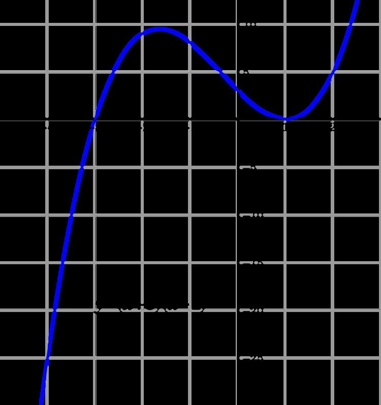
Suppose that we are seeking a zero of the function defined by f(x) = (x + 3)(x − 1)². We take [a₀, b₀] = [−4, 4/3] as our initial interval. We have f(a₀) = −25 and f(b₀) = 0.48148 (all numbers in this section are rounded), so the conditions f(a₀) f(b₀) < 0 and |f(b₀)| ≤ |f(a₀)| are satisfied.

1. In the first iteration, we use linear interpolation between (b₋₁, f(b₋₁)) = (a₀, f(a₀)) = (−4, −25) and (b₀, f(b₀)) = (1.33333, 0.48148), which yields s = 1.23256. This lies between (3a₀ + b₀) / 4 and b₀, so this value is accepted. Furthermore, f(1.23256) = 0.22891, so we set a₁ = a₀ and b₁ = s = 1.23256.
2. In the second iteration, we use inverse quadratic interpolation between (a₁, f(a₁)) = (−4, −25) and (b₀, f(b₀)) = (1.33333, 0.48148) and (b₁, f(b₁)) = (1.23256, 0.22891). This yields 1.14205, which lies between (3a₁ + b₁) / 4 and b₁. Furthermore, the inequality |1.14205 − b₁| ≤ |b₀ − b₋₁| / 2 is satisfied, so this value is accepted. Furthermore, f(1.14205) = 0.083582, so we set a₂ = a₁ and b₂ = 1.14205.
3. In the third iteration, we use inverse quadratic interpolation between (a₂, f(a₂)) = (−4, −25) and (b₁, f(b₁)) = (1.23256, 0.22891) and (b₂, f(b₂)) = (1.14205, 0.083582). This yields 1.09032, which lies between (3a₂ + b₂) / 4 and b₂. But here Brent's additional condition kicks in: the inequality |1.09032 − b₂| ≤ |b₁ − b₀| / 2 is not satisfied, so this value is rejected. Instead, the midpoint m = −1.42897 of the interval [a₂, b₂] is computed. We have f(m) = 9.26891, so we set a₃ = a₂ and b₃ = −1.42897.
4. In the fourth iteration, we use inverse quadratic interpolation between (a₃, f(a₃)) = (−4, −25) and (b₂, f(b₂)) = (1.14205, 0.083582) and (b₃, f(b₃)) = (−1.42897, 9.26891). This yields 1.15448, which is not in the interval between (3a₃ + b₃) / 4 and b₃). Hence, it is replaced by the midpoint m = −2.71449. We have f(m) = 3.93934, so we set a₄ = a₃ and b₄ = −2.71449.
5. In the fifth iteration, inverse quadratic interpolation yields −3.45500, which lies in the required interval. However, the previous iteration was a bisection step, so the inequality |−3.45500 − b₄| ≤ |b₄ − b₃| / 2 need to be satisfied. This inequality is false, so we use the midpoint m = −3.35724. We have f(m) = −6.78239, so m becomes the new contrapoint (a₅ = −3.35724) and the iterate remains the same (b₅ = b₄).
6. In the sixth iteration, we cannot use inverse quadratic interpolation because b₅ = b₄. Hence, we use linear interpolation between (a₅, f(a₅)) = (−3.35724, −6.78239) and (b₅, f(b₅)) = (−2.71449, 3.93934). The result is s = −2.95064, which satisfies all the conditions. But since the iterate did not change in the previous step, we reject this result and fall back to bisection. We update s = -3.03587, and f(s) = -0.58418.
7. In the seventh iteration, we can again use inverse quadratic interpolation. The result is s = −3.00219, which satisfies all the conditions. Now, f(s) = −0.03515, so we set a₇ = b₆ and b₇ = −3.00219 (a₇ and b₇ are exchanged so that the condition |f(b₇)| ≤ |f(a₇)| is satisfied). (Correct : linear interpolation s = -2.99436, f(s) = 0.089961)
8. In the eighth iteration, we cannot use inverse quadratic interpolation because a₇ = b₆. Linear interpolation yields s = −2.99994, which is accepted. (Correct : s = -2.9999, f(s) = 0.0016)
9. In the following iterations, the root x = −3 is approached rapidly: b₉ = −3 + 6·10⁻⁸ and b₁₀ = −3 − 3·10⁻¹⁵. (Correct : Iter 9 : f(s) = -1.4E-07, Iter 10 : f(s) = 6.96E-12)

Implementations

Brent (1973) published an Algol 60 implementation.

Netlib contains a Fortran translation of this implementation with slight modifications.

The PARI/GP method solve implements the method.

Other implementations of the algorithm (in C++, C, and Fortran) can be found in the Numerical Recipes books.

The Apache Commons Math library implements the algorithm in Java.

The SciPy optimize module implements the algorithm in Python (programming language)

The Modelica Standard Library implements the algorithm in Modelica.

The optimize function implements the algorithm in R (software).

The Boost (C++ libraries) implements the algorithm in C++ in the Math toolkit ("Locating function minima").

The Optim.jl package implements the algorithm in Julia (programming language)