Bias–variance tradeoff - Alchetron, The Free Social Encyclopedia

In statistics and machine learning, the bias–variance tradeoff (or dilemma) is the problem of simultaneously minimizing two sources of error that prevent supervised learning algorithms from generalizing beyond their training set:

Motivation

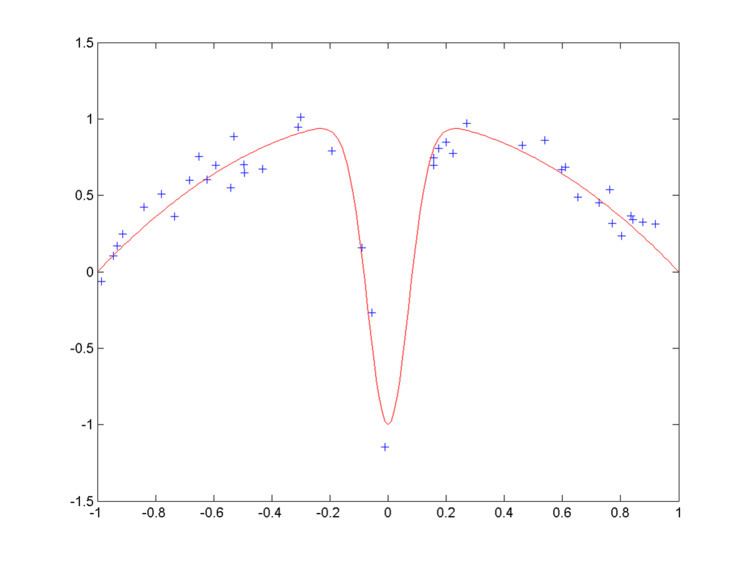
The bias–variance tradeoff is a central problem in supervised learning. Ideally, one wants to choose a model that both accurately captures the regularities in its training data, but also generalizes well to unseen data. Unfortunately, it is typically impossible to do both simultaneously. High-variance learning methods may be able to represent their training set well, but are at risk of overfitting to noisy or unrepresentative training data. In contrast, algorithms with high bias typically produce simpler models that don't tend to overfit, but may underfit their training data, failing to capture important regularities.

Models with low bias are usually more complex (e.g. higher-order regression polynomials), enabling them to represent the training set more accurately. In the process, however, they may also represent a large noise component in the training set, making their predictions less accurate - despite their added complexity. In contrast, models with higher bias tend to be relatively simple (low-order or even linear regression polynomials), but may produce lower variance predictions when applied beyond the training set.

Bias–variance decomposition of squared error

Suppose that we have a training set consisting of a set of points x 1 , … , x n and real values y i associated with each point x i . We assume that there is a function with noise y = f ( x ) + ϵ , where the noise, ϵ , has zero mean and variance σ 2 .

We want to find a function f ^ ( x ) , that approximates the true function f ( x ) as well as possible, by means of some learning algorithm. We make "as well as possible" precise by measuring the mean squared error between y and f ^ ( x ) : we want ( y − f ^ ( x ) ) 2 to be minimal, both for x 1 , … , x n and for points outside of our sample. Of course, we cannot hope to do so perfectly, since the y i contain noise ϵ ; this means we must be prepared to accept an irreducible error in any function we come up with.

Finding an f ^ that generalizes to points outside of the training set can be done with any of the countless algorithms used for supervised learning. It turns out that whichever function f ^ we select, we can decompose its expected error on an unseen sample x as follows:

E [ ( y − f ^ ( x ) ) 2 ] = B i a s [ f ^ ( x ) ] 2 + V a r [ f ^ ( x ) ] + σ 2

Where:

B i a s [ f ^ ( x ) ] = E [ f ^ ( x ) − f ( x ) ]

and

V a r [ f ^ ( x ) ] = E [ f ^ ( x ) 2 ] − E [ f ^ ( x ) ] 2

The expectation ranges over different choices of the training set x 1 , … , x n , y 1 , … , y n , all sampled from the same joint distribution P ( x , y ) . The three terms represent:

the square of the bias of the learning method, which can be thought of as the error caused by the simplifying assumptions built into the method. E.g., when approximating a non-linear function f ( x ) using a learning method for linear models, there will be error in the estimates f ^ ( x ) due to this assumption;

the variance of the learning method, or, intuitively, how much the learning method f ^ ( x ) will move around its mean;

the irreducible error σ 2 . Since all three terms are non-negative, this forms a lower bound on the expected error on unseen samples.

The more complex the model f ^ ( x ) is, the more data points it will capture, and the lower the bias will be. However, complexity will make the model "move" more to capture the data points, and hence its variance will be larger.

Derivation

The derivation of the bias–variance decomposition for squared error proceeds as follows. For notational convenience, abbreviate f = f ( x ) and f ^ = f ^ ( x ) . First, note that for any random variable X , we have

V a r [ X ] = E [ X 2 ] − E [ X ] 2

Rearranging, we get:

E [ X 2 ] = V a r [ X ] + E [ X ] 2

Since f is deterministic

E [ f ] = f .

This, given y = f + ϵ and E [ ϵ ] = 0 , implies E [ y ] = E [ f + ϵ ] = E [ f ] = f .

Also, since V a r [ ϵ ] = σ 2

V a r [ y ] = E [ ( y − E [ y ] ) 2 ] = E [ ( y − f ) 2 ] = E [ ( f + ϵ − f ) 2 ] = E [ ϵ 2 ] = V a r [ ϵ ] + E [ ϵ ] 2 = σ 2

Thus, since ϵ and f ^ are independent, we can write

E [ ( y − f ^ ) 2 ] = E [ y 2 + f ^ 2 − 2 y f ^ ] = E [ y 2 ] + E [ f ^ 2 ] − E [ 2 y f ^ ] = V a r [ y ] + E [ y ] 2 + V a r [ f ^ ] + E [ f ^ ] 2 − 2 f E [ f ^ ] = V a r [ y ] + V a r [ f ^ ] + ( f 2 − 2 f E [ f ^ ] + E [ f ^ ] 2 ) = V a r [ y ] + V a r [ f ^ ] + ( f − E [ f ^ ] ) 2 = V a r [ y ] + V a r [ f ^ ] + E [ f − f ^ ] 2 = σ 2 + V a r [ f ^ ] + B i a s [ f ^ ] 2

Application to regression

The bias-variance decomposition forms the conceptual basis for regression regularization methods such as Lasso and Ridge Regression. Regularization methods introduce bias into the regression solution that can reduce variance considerably relative to the OLS solution. Although the OLS solution provides non-biased regression estimates, the lower variance solutions produced by regularization techniques provide superior MSE performance.

Application to classification

The bias–variance decomposition was originally formulated for least-squares regression. For the case of classification under the 0-1 loss (misclassification rate), it's possible to find a similar decomposition. Alternatively, if the classification problem can be phrased as probabilistic classification, then the expected squared error of the predicted probabilities with respect to the true probabilities can be decomposed as before.

Approaches

Dimensionality reduction and feature selection can decrease variance by simplifying models. Similarly, a larger training set tends to decrease variance. Adding features (predictors) tends to decrease bias, at the expense of introducing additional variance. Learning algorithms typically have some tunable parameters that control bias and variance, e.g.:

(Generalized) linear models can be regularized to decrease their variance at the cost of increasing their bias.

In artificial neural networks, the variance increases and the bias decreases with the number of hidden units. Like in GLMs, regularization is typically applied.

In k-nearest neighbor models, a high value of k leads to high bias and low variance (see below).

In Instance-based learning, regularization can be achieved varying the mixture of prototypes and exemplars.

In decision trees, the depth of the tree determines the variance. Decision trees are commonly pruned to control variance.

One way of resolving the trade-off is to use mixture models and ensemble learning. For example, boosting combines many "weak" (high bias) models in an ensemble that has lower bias than the individual models, while bagging combines "strong" learners in a way that reduces their variance.

K-nearest neighbors

In the case of k-nearest neighbors regression, a closed-form expression exists that relates the bias–variance decomposition to the parameter k:

E [ ( y − f ^ ( x ) ) 2 ] = ( f ( x ) − 1 k ∑ i = 1 k f ( N i ( x ) ) ) 2 + σ 2 k + σ 2

where N 1 ( x ) , … , N k ( x ) are the k nearest neighbors of x in the training set. The bias (first term) is a monotone rising function of k, while the variance (second term) drops off as k is increased. In fact, under "reasonable assumptions" the bias of the first-nearest neighbor (1-NN) estimator vanishes entirely as the size of the training set approaches infinity.

Application to human learning

While widely discussed in the context of machine learning, the bias-variance dilemma has been examined in the context of human cognition, most notably by Gerd Gigerenzer and co-workers in the context of learned heuristics. They have argued (see references below) that the human brain resolves the dilemma in the case of the typically sparse, poorly-characterised training-sets provided by experience by adopting high-bias/low variance heuristics. This reflects the fact that a zero-bias approach has poor generalisability to new situations, and also unreasonably presumes precise knowledge of the true state of the world. The resulting heuristics are relatively simple, but produce better inferences in a wider variety of situations.

Geman et al. argue that the bias-variance dilemma implies that abilities such as generic object recognition cannot be learned from scratch, but require a certain degree of “hard wiring” that is later tuned by experience. This is because model-free approaches to inference require impractically large training sets if they are to avoid high variance.

References

Bias–variance tradeoff Wikipedia

(Text) CC BY-SA

Contents