
 | ||
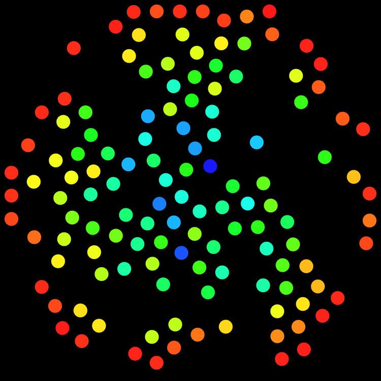
In graph theory, betweenness centrality is a measure of centrality in a graph based on shortest paths. For every pair of vertices in a graph, there exists a shortest path between the vertices such that either the number of edges that the path passes through (for undirected graphs) or the sum of the weights of the edges (for directed graphs) is minimized. The betweenness centrality for each vertex is the number of these shortest paths that pass through the vertex.
Contents
Betweenness centrality finds wide application in network theory: it represents the degree of which nodes stand between each other. For example, in a telecommunications network, a node with higher betweenness centrality would have more control over the network, because more information will pass through that node. Betweenness centrality was devised as a general measure of centrality: it applies to a wide range of problems in network theory, including problems related to social networks, biology, transport and scientific cooperation.
Although earlier authors have intuitively described centrality as based on betweenness, Freeman (1977) gave the first formal definition of betweenness centrality. The idea was earlier proposed by mathematician J. Anthonisse, but his work was never published.
Definition
The betweenness centrality of a node
where
Note that the betweenness centrality of a node scales with the number of pairs of nodes as implied by the summation indices. Therefore, the calculation may be rescaled by dividing through by the number of pairs of nodes not including
which results in:
Note that this will always be a scaling from a smaller range into a larger range, so no precision is lost.
Weighted networks
In a weighted network the links connecting the nodes are no longer treated as binary interactions, but are weighted in proportion to their capacity, influence, frequency, etc., which adds another dimension of heterogeneity within the network beyond the topological effects. A node's strength in a weighted network is given by the sum of the weights of its adjacent edges.
With
A study of the average value
Algorithms
Calculating the betweenness and closeness centralities of all the vertices in a graph involves calculating the shortest paths between all pairs of vertices on a graph, which takes
In calculating betweenness and closeness centralities of all vertices in a graph, it is assumed that graphs are undirected and connected with the allowance of loops and multiple edges. When specifically dealing with network graphs, often graphs are without loops or multiple edges to maintain simple relationships (where edges represent connections between two people or vertices). In this case, using Brandes' algorithm will divide final centrality scores by 2 to account for each shortest path being counted twice.
Another algorithm generalizes the Freeman's betweenness computed on geodesics and Newman's betweenness computed on all paths, by introducing a hyper-parameter controlling the trade-off between exploration and exploitation. The time complexity is the number of edges times the number of nodes in the graph.
The concept of centrality was extended to a group level as well. Group betweenness centrality shows the proportion of geodesics connecting pairs of non-group members that pass through a group of nodes. Brandes' algorithm for computing the betweenness centrality of all vertices was modified to compute the group betweenness centrality of one group of nodes with the same asymptotic running time.
Related concepts
Betweenness centrality is related to a network's connectivity, in so much as high betweenness vertices have the potential to disconnect graphs if removed (see cut set) .