Beta binomial distribution - Alchetron, the free social encyclopedia

Support k ∈ { 0, …, n }

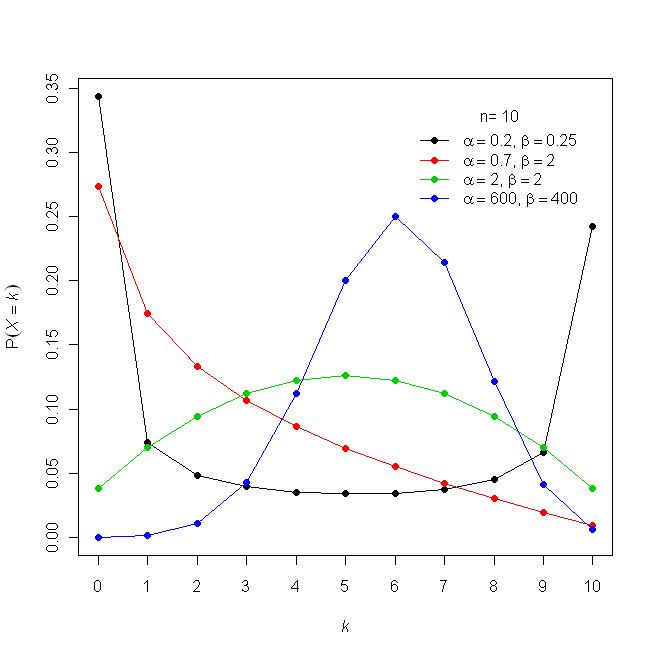Parameters n ∈ N0 — number of trials α > 0 {\displaystyle \alpha >0} (real) β > 0 {\displaystyle \beta >0} (real) pmf ( n k ) B ( k + α , n − k + β ) B ( α , β ) {\displaystyle {n \choose k}{\frac {\mathrm {B} (k+\alpha ,n-k+\beta )}{\mathrm {B} (\alpha ,\beta )}}\!} CDF 1 − B ( β + n − k − 1 , α + k + 1 ) 3 F 2 ( a , b ; k ) B ( α , β ) B ( n − k , k + 2 ) ( n + 1 ) {\displaystyle 1-{\tfrac {\mathrm {B} (\beta +n-k-1,\alpha +k+1)_{3}F_{2}({\boldsymbol {a}},{\boldsymbol {b}};k)}{\mathrm {B} (\alpha ,\beta )\mathrm {B} (n-k,k+2)(n+1)}}} where 3F2(a,b,k) is the generalized hypergeometric function =3F2(1, α + k + 1, −n + k + 1; k + 2, −β − n + k + 2; 1) Mean n α α + β {\displaystyle {\frac {n\alpha }{\alpha +\beta }}\!} Variance n α β ( α + β + n ) ( α + β ) 2 ( α + β + 1 ) {\displaystyle {\frac {n\alpha \beta (\alpha +\beta +n)}{(\alpha +\beta )^{2}(\alpha +\beta +1)}}\!}

In probability theory and statistics, the beta-binomial distribution is a family of discrete probability distributions on a finite support of non-negative integers arising when the probability of success in each of a fixed or known number of Bernoulli trials is either unknown or random. The beta-binomial distribution is the binomial distribution in which the probability of success at each trial is not fixed but random and follows the beta distribution. It is frequently used in Bayesian statistics, empirical Bayes methods and classical statistics to capture overdispersion in binomial type distributed data.

It reduces to the Bernoulli distribution as a special case when n = 1. For α = β = 1, it is the discrete uniform distribution from 0 to n. It also approximates the binomial distribution arbitrarily well for large α and β. The beta-binomial is a one-dimensional version of the Dirichlet-multinomial distribution, as the binomial and beta distributions are univariate versions of the multinomial and Dirichlet distributions, respectively.

Beta-binomial distribution as a compound distribution

The Beta distribution is a conjugate distribution of the binomial distribution. This fact leads to an analytically tractable compound distribution where one can think of the p parameter in the binomial distribution as being randomly drawn from a beta distribution. Namely, if

X ∼ Bin ⁡ ( n , p )

then

P ( X = k | p , n ) = L ( p | k ) = ( n k ) p k ( 1 − p ) n − k

where Bin(n,p) stands for the binomial distribution, and where p is a random variable with a beta distribution.

π ( p | α , β ) = B e t a ( α , β ) = p α − 1 ( 1 − p ) β − 1 B ( α , β )

then the compound distribution is given by

f ( k | n , α , β ) = ∫ 0 1 L ( p | k ) π ( p | α , β ) d p = ( n k ) 1 B ( α , β ) ∫ 0 1 p k + α − 1 ( 1 − p ) n − k + β − 1 d p = ( n k ) B ( k + α , n − k + β ) B ( α , β ) .

Using the properties of the beta function, this can alternatively be written

f ( k | n , α , β ) = Γ ( n + 1 ) Γ ( k + 1 ) Γ ( n − k + 1 ) Γ ( k + α ) Γ ( n − k + β ) Γ ( n + α + β ) Γ ( α + β ) Γ ( α ) Γ ( β ) .

Beta-binomial as an urn model

The beta-binomial distribution can also be motivated via an urn model for positive integer values of α and β, known as the Polya urn model. Specifically, imagine an urn containing α red balls and β black balls, where random draws are made. If a red ball is observed, then two red balls are returned to the urn. Likewise, if a black ball is drawn, then two black balls are returned to the urn. If this is repeated n times, then the probability of observing k red balls follows a beta-binomial distribution with parameters n,α and β.

Note that if the random draws are with simple replacement (no balls over and above the observed ball are added to the urn), then the distribution follows a binomial distribution and if the random draws are made without replacement, the distribution follows a hypergeometric distribution.

Moments and properties

The first three raw moments are

and the kurtosis is

Letting π = α α + β we note, suggestively, that the mean can be written as

and the variance as

where ρ = 1 α + β + 1 . The parameter ρ is known as the "intra class" or "intra cluster" correlation. It is this positive correlation which gives rise to overdispersion.

The following recurrence relation holds:

{ ( α + k ) ( n − k ) p ( k ) − ( k + 1 ) p ( k + 1 ) ( β − k + n − 1 ) = 0 , p ( 0 ) = ( β ) n ( α + β ) n }

Method of moments

The method of moments estimates can be gained by noting the first and second moments of the beta-binomial namely

and setting these raw moments equal to the first and second raw sample moments respectively

and solving for α and β we get

Note that these estimates can be non-sensically negative which is evidence that the data is either undispersed or underdispersed relative to the binomial distribution. In this case, the binomial distribution and the hypergeometric distribution are alternative candidates respectively.

Maximum likelihood estimation

While closed-form maximum likelihood estimates are impractical, given that the pdf consists of common functions (gamma function and/or Beta functions), they can be easily found via direct numerical optimization. Maximum likelihood estimates from empirical data can be computed using general methods for fitting multinomial Pólya distributions, methods for which are described in (Minka 2003). The R package VGAM through the function vglm, via maximum likelihood, facilitates the fitting of glm type models with responses distributed according to the beta-binomial distribution. Note also that there is no requirement that n is fixed throughout the observations.

Example

The following data gives the number of male children among the first 12 children of family size 13 in 6115 families taken from hospital records in 19th century Saxony (Sokal and Rohlf, p. 59 from Lindsey). The 13th child is ignored to assuage the effect of families non-randomly stopping when a desired gender is reached.

We note the first two sample moments are

and therefore the method of moments estimates are

The maximum likelihood estimates can be found numerically

and the maximized log-likelihood is

from which we find the AIC

The AIC for the competing binomial model is AIC = 25070.34 and thus we see that the beta-binomial model provides a superior fit to the data i.e. there is evidence for overdispersion. Trivers and Willard posit a theoretical justification for heterogeneity (also known as "burstiness") in gender-proneness among mammalian offspring (i.e. overdispersion).

The superior fit is evident especially among the tails

Further Bayesian considerations

It is convenient to reparameterize the distributions so that the expected mean of the prior is a single parameter: Let

π ( θ | μ , M ) = Beta ⁡ ( M μ , M ( 1 − μ ) ) = Γ ( M ) Γ ( M μ ) Γ ( M ( 1 − μ ) ) θ M μ − 1 ( 1 − θ ) M ( 1 − μ ) − 1

where

so that

The posterior distribution ρ(θ|k) is also a beta distribution:

ρ ( θ | k ) ∝ ℓ ( k | θ ) π ( θ | μ , M ) = Beta ⁡ ( k + M μ , n − k + M ( 1 − μ ) ) = Γ ( M ) Γ ( M μ ) Γ ( M ( 1 − μ ) ) ( n k ) θ k + M μ − 1 ( 1 − θ ) n − k + M ( 1 − μ ) − 1

And

E ⁡ ( θ | k ) = k + M μ n + M .

while the marginal distribution m(k|μ, M) is given by

m ( k | μ , M ) = ∫ 0 1 l ( k | θ ) π ( θ | μ , M ) d θ = Γ ( M ) Γ ( M μ ) Γ ( M ( 1 − μ ) ) ( n k ) ∫ 0 1 θ k + M μ − 1 ( 1 − θ ) n − k + M ( 1 − μ ) − 1 d θ = Γ ( M ) Γ ( M μ ) Γ ( M ( 1 − μ ) ) ( n k ) Γ ( k + M μ ) Γ ( n − k + M ( 1 − μ ) ) Γ ( n + M ) .

Substituting back M and μ, in terms of α and β , this becomes:

m ( k | α , β ) = Γ ( n + 1 ) Γ ( k + 1 ) Γ ( n − k + 1 ) Γ ( k + α ) Γ ( n − k + β ) Γ ( n + α + β ) Γ ( α + β ) Γ ( α ) Γ ( β ) .

which is the expected beta-binomial distribution with parameters n , α and β .

We can also use the method of iterated expectations to find the expected value of the marginal moments. Let us write our model as a two-stage compound sampling model. Let k_i be the number of success out of n_i trials for event i:

We can find iterated moment estimates for the mean and variance using the moments for the distributions in the two-stage model:

(Here we have used the law of total expectation and the law of total variance.)

We want point estimates for μ and M . The estimated mean μ ^ is calculated from the sample

The estimate of the hyperparameter M is obtained using the moment estimates for the variance of the two-stage model:

Solving:

where

Since we now have parameter point estimates, μ ^ and M ^ , for the underlying distribution, we would like to find a point estimate θ ~ i for the probability of success for event i. This is the weighted average of the event estimate θ i ^ = k i / n i and μ ^ . Given our point estimates for the prior, we may now plug in these values to find a point estimate for the posterior

Shrinkage factors

We may write the posterior estimate as a weighted average:

where B ^ i is called the shrinkage factor.

B B ( 1 , 1 , n ) ∼ U ( 0 , n ) where U ( a , b ) is the discrete uniform distribution.

References

Beta-binomial distribution Wikipedia

(Text) CC BY-SA

Eric Potts

Vladan Savić

Contents