Bayesian estimation of templates in computational anatomy

The deformable template model of shapes and forms via diffeomorphic group actions

Linear algebra is one of the central tools to modern engineering. Central to linear algebra is the notion of an orbit of vectors, with the matrices forming groups (matrices with inverses and identity) which act on the vectors. In linear algebra the equations describing the orbit elements the vectors are linear in the vectors being acted upon by the matrices. In computational anatomy the space of all shapes and forms is modeled as an orbit similar to the vectors in linear-algebra, however the groups do not act linear as the matrices do, and the shapes and forms are not additive. In computational anatomy addition is essentially replaced by the law of composition.

The central group acting CA defined on volumes in R 3 are the diffeomorphisms G ≐ D i f f which are mappings with 3-components ϕ ( ⋅ ) = ( ϕ 1 ( ⋅ ) , ϕ 2 ( ⋅ ) , ϕ 3 ( ⋅ ) ) , law of composition of functions ϕ ∘ ϕ ′ ( ⋅ ) ≐ ϕ ( ϕ ′ ( ⋅ ) ) , with inverse ϕ ∘ ϕ − 1 ( ⋅ ) = ϕ ( ϕ − 1 ( ⋅ ) ) = i d .

Groups and group are familiar to the Engineering community with the universal popularization and standardization of linear algebra as a basic model

A popular group action is on scalar images, I ( x ) , x ∈ R 3 , with action on the right via the inverse.

For sub-manifolds X ⊂ R 3 ∈ M , parametrized by a chart or immersion m ( u ) , u ∈ U , the diffeomorphic action the flow of the position

Several group actions in computational anatomy have been defined.

Geodesic positioning via the Riemannian exponential

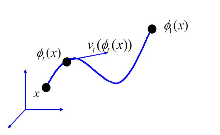
For the study of deformable shape in CA, a more general diffeomorphism group has been the group of choice, which is the infinite dimensional analogue. The high-dimensional diffeomorphism groups used in computational anatomy are generated via smooth flows ϕ t , t ∈ [ 0 , 1 ] which satisfy the Lagrangian and Eulerian specification of the flow fields satisfying the ordinary differential equation:

with v ≐ ( v 1 , v 2 , v 3 ) the vector fields on R 3 termed the Eulerian velocity of the particles at position ϕ of the flow. The vector fields are functions in a function space, modelled as a smooth Hilbert space with the vector fields having 1-continuous derivative . For v t = ϕ ˙ t ∘ ϕ t − 1 , t ∈ [ 0 , 1 ] , with the inverse for the flow given by

and the 3 × 3 Jacobian matrix for flows in R 3 given as   D ϕ ≐ ( ∂ ϕ i ∂ x j ) .

Flows were first introduced for large deformations in image matching; ϕ ˙ t ( x ) is the instantaneous velocity of particle x at time t . with the vector fields termed the Eulerian velocity of the particles at position of the flow. The modelling approach used in CA enforces a continuous differentiability condition on the vector fields by modelling the space of vector fields ( V , ∥ ⋅ ∥ V ) as a reproducing kernel Hilbert space (RKHS), with the norm defined by a 1-1, differential operator A : V → V ∗ , Green's inverse K = A − 1 . The norm according to ∥ v ∥ V 2 ≐ ∫ X A v ⋅ v d x , v ∈ V , where for σ ( v ) ≐ A v ∈ V ∗ a generalized function or distribution, then ( σ ∣ w ) ≐ ∫ R 3 ∑ i w i ( x ) σ i ( d x ) . Since A is a differential operator, finiteness of the norm-square ∫ X A v ⋅ v d x < ∞ includes derivatives from the differential operator implying smoothness of the vector fields.

To ensure smooth flows of diffeomorphisms with inverse, the vector fields R 3 must be at least 1-time continuously differentiable in space which are modelled as elements of the Hilbert space ( V , ∥ ⋅ ∥ V ) using the Sobolev embedding theorems so that each element v i ∈ H 0 3 , i = 1 , 2 , 3 , has 3-square-integrable derivatives. Thus ( V , ∥ ⋅ ∥ V ) embed smoothly in 1-time continuously differentiable functions. The diffeomorphism group are flows with vector fields absolutely integrable in Sobolev norm:

The Bayes model of computational anatomy

The central statistical model of computational anatomy in the context of medical imaging is the source-channel model of Shannon theory; the source is the deformable template of images I ∈ I , the channel outputs are the imaging sensors with observables I D ∈ I D . The variation in the anatomical configurations are modelled separately from the Medical imaging modalities Computed Axial Tomography machine, MRI machine, PET machine, and others. The Bayes theory models the prior on the source of images π I ( ⋅ ) on I ∈ I , and the conditional density on the observable imagery p ( ⋅ | I )   on   I D ∈ I D , conditioned on I ∈ I . For images with diffeomorphism group action I ≐ ϕ ⋅ I t e m p , ϕ ∈ D i f f V , then the prior on the group π D i f f V ( ⋅ ) induces the prior on images π I ( ⋅ ) , written as densities the log-posterior takes the form

Maximum a posteriori estimation (MAP) estimation is central to modern statistical theory. Parameters of interest θ ∈ Θ take many forms including (i) disease type such as neurodegenerative or neurodevelopmental diseases, (ii) structure type such as cortical or subcorical structures in problems associated to segmentation of images, and (iii) template reconstruction from populations. Given the observed image I D , MAP estimation maximizes the posterior:

This requires computation of the conditional probabilities p ( θ ∣ I D ) = p ( I D , θ ) p ( I D ) . The multiple atlas orbit model randomizes over the denumerable set of atlases { I a , a ∈ A } . The model on images in the orbit take the form of a multi-modal mixture distribution

Surface templates for computational neuroanatomy and subcortical structures

The study of sub-cortical neroanatomy has been the focus of many studies. Since the original publications by Csernansky and colleagues of hippocampal change in Schizophrenia, Alzheimer's disease, and Depression, many neuroanatomical shape statistical studies have now been completed using templates built from all of the subcortical structures for depression, Alzheimer's, Bipolar disorder, ADHD, autism, and Huntington's Disease. Templates were generated using Bayesian template estimation data back to Ma, Younes and Miller.

Shown in the accompanying Figure is an example of subcortical structure templates generated from T1-weighted magnetic resonance imagery by Tang et al. for the study of Alzheimer's disease in the ADNI population of subjects.

Surface estimation in cardiac computational anatomy

Numerous studies have now been done on cardiac hypertrophy and the role of the structural integraties in the functional mechanics of the heart. Siamak Ardekani has been working on populations of Cardiac anatomies reconstructing atlas coordinate systems from populations. The figure on the right shows the computational cardiac anatomy method being used to identify regional differences in radial thickness at end-systolic cardiac phase between patients with hypertrophic cardiomyopathy (left) and hypertensive heart disease (right). Color map that is placed on a common surface template (gray mesh) represents region ( basilar septal and the anterior epicardial wall) that has on average significantly larger radial thickness in patients with hypertrophic cardiomyopathy vs. hypertensive heart disease (reference below).

MAP Estimation of volume templates from populations and the EM algorithm

Generating templates empirically from populations is a fundamental operation ubiquitous to the discipline. Several methods based on Bayesian statistics have emerged for submanifolds and dense image volumes. For the dense image volume case, given the observable I D 1 , I D 2 , … the problem is to estimate the template in the orbit of dense images I ∈ I . Ma's procedure takes an initial hypertemplate I 0 ∈ I as the starting point, and models the template in the orbit under the unknown to be estimated diffeomorphism I ≐ ϕ 0 ⋅ I 0 , with the parameters to be estimated the log-coordinates θ ≐ v 0 determining the geodesic mapping of the hyper-template E x p i d ( v 0 ) ⋅ I 0 = I ∈ I .

In the Bayesian random orbit model of computational anatomy the observed MRI images I D i are modelled as a conditionally Gaussian random field with mean field ϕ i ⋅ I , with ϕ i a random unknown transformation of the template. The MAP estimation problem is to estimate the unknown template I ∈ I given the observed MRI images.

Ma's procedure for dense imagery takes an initial hypertemplate I 0 ∈ I as the starting point, and models the template in the orbit under the unknown to be estimated diffeomorphism I ≐ ϕ 0 ⋅ I 0 . The observables are modelled as conditional random fields, I D i a conditional-Gaussian random field with mean field ϕ i ⋅ I ≐ ϕ i ⋅ ϕ 0 ⋅ I 0 . The unknown variable to be estimated explicitly by MAP is the mapping of the hyper-template ϕ 0 , with the other mappings considered as nuisance or hidden variables which are integrated out via the Bayes procedure. This is accomplished using the expectation-maximization (EM) algorithm.

The orbit-model is exploited by associating the unknown to be estimated flows to their log-coordinates v i , i = 1 , … via the Riemannian geodesic log and exponential for computational anatomy the initial vector field in the tangent space at the identity so that E x p i d ( v i ) ≐ ϕ i , with E x p i d ( v 0 ) the mapping of the hyper-template. The MAP estimation problem becomes

The EM algorithm takes as complete data the vector-field coordinates parameterizing the mapping, v i , i = 1 , … and compute iteratively the conditional-expectation