Backpressure routing

Introduction to backpressure routing

Backpressure routing is an algorithm for dynamically routing traffic over a multi-hop network by using congestion gradients. The algorithm can be applied to wireless communication networks, including sensor networks, mobile ad hoc networks (MANETS), and heterogeneous networks with wireless and wireline components . Backpressure principles can also be applied to other areas, such as to the study of product assembly systems and processing networks . This article focuses on communication networks, where packets from multiple data streams arrive and must be delivered to appropriate destinations. The backpressure algorithm operates in slotted time. Every time slot it seeks to route data in directions that maximize the differential backlog between neighboring nodes. This is similar to how water flows through a network of pipes via pressure gradients. However, the backpressure algorithm can be applied to multi-commodity networks (where different packets may have different destinations), and to networks where transmission rates can be selected from a set of (possibly time-varying) options. Attractive features of the backpressure algorithm are: (i) it leads to maximum network throughput, (ii) it is provably robust to time-varying network conditions, (iii) it can be implemented without knowing traffic arrival rates or channel state probabilities. However, the algorithm may introduce large delays, and may be difficult to implement exactly in networks with interference. Modifications of backpressure that reduce delay and simplify implementation are described below under Improving delay and Distributed backpressure.

Backpressure routing has mainly been studied in a theoretical context. In practice, ad hoc wireless networks have typically implemented alternative routing methods based on shortest path computations or network flooding, such as Ad Hoc on-Demand Distance Vector Routing (AODV), geographic routing, and extremely opportunistic routing (ExOR). However, the mathematical optimality properties of backpressure have motivated recent experimental demonstrations of its use on wireless testbeds at the University of Southern California and at North Carolina State University .

Origins

The original backpressure algorithm was developed by Tassiulas and Ephremides. They considered a multi-hop packet radio network with random packet arrivals and a fixed set of link selection options. Their algorithm consisted of a max-weight link selection stage and a differential backlog routing stage. An algorithm related to backpressure, designed for computing multi-commodity network flows, was developed in Awerbuch and Leighton. The backpressure algorithm was later extended by Neely, Modiano, and Rohrs to treat scheduling for mobile networks. Backpressure is mathematically analyzed via the theory of Lyapunov drift, and can be used jointly with flow control mechanisms to provide network utility maximization. (see also Backpressure with Utility Optimization and Penalty Minimization).

How it works

Backpressure routing is designed to make decisions that (roughly) minimize the sum of squares of queue backlogs in the network from one timeslot to the next. The precise mathematical development of this technique is described in later sections. This section describes the general network model and the operation of backpressure routing with respect to this model.

The multi-hop queueing network model

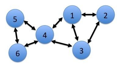
Consider a multi-hop network with N nodes (see Fig. 1 for an example with N = 6). The network operates in slotted time t ∈ { 0 , 1 , 2 , … } . On each slot, new data can arrive to the network, and routing and transmission scheduling decisions are made in an effort to deliver all data to its proper destination. Let data that is destined for node c ∈ { 1 , … , N } be labeled as commodity c data. Data in each node is stored according to its commodity. For n ∈ { 1 , … , N } and c ∈ { 1 , … , N } , let Q n ( c ) ( t ) be the current amount of commodity c data in node n, also called the queue backlog. A closeup of the queue backlogs inside a node is shown in Fig. 2. The units of Q n ( c ) ( t ) depend on the context of the problem. For example, backlog can take integer units of packets, which is useful in cases when data is segmented into fixed length packets. Alternatively, it can take real valued units of bits. It is assumed that Q c ( c ) ( t ) = 0 for all c ∈ { 1 , … , N } and all timeslots t, because no node stores data destined for itself. Every timeslot, nodes can transmit data to others. Data that is transmitted from one node to another node is removed from the queue of the first node and added to the queue of the second. Data that is transmitted to its destination is removed from the network. Data can also arrive exogenously to the network, and A n ( c ) ( t ) is defined as the amount of new data that arrives to node n on slot t that must eventually be delivered to node c.

Let μ a b ( t ) be the transmission rate used by the network over link (a,b) on slot t, representing the amount of data it can transfer from node a to node b on the current slot. Let ( μ a b ( t ) ) be the transmission rate matrix. These transmission rates must be selected within a set of possibly time-varying options. Specifically, the network may have time-varying channels and node mobility, and this can affect its transmission capabilities every slot. To model this, let S(t) represent the topology state of the network, which captures properties of the network on slot t that affect transmission. Let Γ S ( t ) represent the set of transmission rate matrix options available under topology state S(t). Every slot t, the network controller observes S(t) and chooses transmission rates ( μ a b ( t ) ) within the set Γ S ( t ) . The choice of which ( μ a b ( t ) ) matrix to select on each slot t is described in the next subsection.

This time-varying network model was first developed for the case when transmission rates every slot t were determined by general functions of a channel state matrix and a power allocation matrix. The model can also be used when rates are determined by other control decisions, such as server allocation, sub-band selection, coding type, and so on. It assumes the supportable transmission rates are known and there are no transmission errors. Extended formulations of backpressure routing can be used for networks with probabilistic channel errors, including networks that exploit the wireless broadcast advantage via multi-receiver diversity.

The backpressure control decisions

Every slot t the backpressure controller observes S(t) and performs the following 3 steps:

Choosing the optimal commodity

Each node a observes its own queue backlogs and the backlogs in its current neighbors. A current neighbor of node a is a node b such that it is possible to choose a non-zero transmission rate μ a b ( t ) on the current slot. Thus, neighbors are determined by the set Γ S ( t ) . In the extreme case, a node can have all N − 1 other nodes as neighbors. However, it is common to use sets Γ S ( t ) that preclude transmissions between nodes that are separated by more than a certain geographic distance, or that would have a propagated signal strength below a certain threshold. Thus, it is typical for the number of neighbors to be much less than N − 1. The example in Fig. 1 illustrates neighbors by link connections, so that node 5 has neighbors 4 and 6. The example suggests a symmetric relationship between neighbors (so that if 5 is a neighbor of 4, then 4 is a neighbor of 5), but this need not be the case in general.

The set of neighbors of a given node determines the set of outgoing links it can use for transmission on the current slot. For each outgoing link (a,b), the optimal commodity c a b o p t ( t ) is defined as the commodity c ∈ { 1 , … , N } that maximizes the following differential backlog quantity:

Any ties in choosing the optimal commodity are broken arbitrarily.

An example is shown in Fig. 2. The example assumes each queue currently has only 3 commodities: red, green, and blue, and these are measured in integer units of packets. Focusing on the directed link (1,2), the differential backlogs are:

Hence, the optimal commodity to send over link (1,2) on slot t is the green commodity. On the other hand, the optimal commodity to send over the reverse link (2,1) on slot t is the blue commodity.

Choosing the μab(t) matrix

Once the optimal commodities have been determined for each link (a,b), the network controller computes the following weights W a b ( t ) :

The weight W a b ( t ) is the value of the differential backlog associated with the optimal commodity for link (a,b), maxed with 0. The controller then chooses transmission rates as the solution to the following max-weight problem (breaking ties arbitrarily):

As an example of the max-weight decision, suppose that on the current slot t, the differential backlogs on each link of the 6 node network lead to link weights W a b ( t ) given by:

While the set Γ S ( t ) might contain an uncountably infinite number of possible transmission rate matrices, assume for simplicity that the current topology state admits only 4 possible choices:

illustration of the 4 possible transmission rate selections under the current topology state S(t). Option (a) activates the single link (1,5) with a transmission rate of μ 15 = 2 . All other options use two links, with transmission rates of 1 on each of the activated links.]]

These four possibilities are illustrated in Fig. 3. The options in Fig. 3 are represented in matrix form by:

Observe that node 6 can neither send nor receive under any of these possibilities. This might arise because node 6 is currently out of communication range. The weighted sum of rates for each of the 4 possibilities are:

Because there is a tie for the maximum weight of 12, the network controller can break the tie arbitrarily by choosing either option μ a or option μ d .

Finalizing the routing variables

Suppose now that the optimal commodities c a b o p t ( t ) have been determined for each link, and the transmission rates ( μ a b ( t ) ) have also been determined. If the differential backlog for the optimal commodity on a given link (a,b) is negative, then no data is transferred over this link on the current slot. Else, the network offers to send μ a b ( t ) units of commodity c a b o p t ( t ) data over this link. This is done by defining routing variables μ a b ( c ) ( t ) for each link (a,b) and each commodity c, where:

The value of μ a b ( c ) ( t ) represents the transmission rate offered to commodity c data over link (a,b) on slot t. However, nodes might not have enough of a certain commodity to support transmission at the offered rates on all of their outgoing links. This arises on slot t for node n and commodity c if:

In this case, all of the Q n ( c ) ( t ) data is sent, and null data is used to fill the unused portions of the offered rates, allocating the actual data and null data arbitrarily over the corresponding outgoing links (according to the offered rates). This is called a queue underflow situation. Such underflows do not affect the throughput or stability properties of the network. Intuitively, this is because underflows only arise when the transmitting node has a low amount of backlog, which means the node is not in danger of instability.

Improving delay

It is important to note that the backpressure algorithm does not use any pre-specified paths. Paths are learned dynamically, and may be different for different packets. Delay can be very large, particularly when the system is lightly loaded so that there is not enough pressure to push data towards the destination. As an example, suppose one packet enters the network, and nothing else ever enters. This packet may take a loopy walk through the network and never arrive at its destination because no pressure gradients build up. This does not contradict the throughput optimality or stability properties of backpressure because the network has at most one packet at any time and hence is trivially stable (achieving a delivery rate of 0, equal to the arrival rate).

It is also possible to implement backpressure on a set of pre-specified paths. This can restrict the capacity region, but might improve in-order delivery and delay. Another way to improve delay, without affecting the capacity region, is to use an enhanced version that biases link weights towards desirable directions. Simulations of such biasing have shown significant delay improvements. Note that backpressure does not require First-in-First-Out (FIFO) service at the queues. It has been observed that Last-in-First-Out (LIFO) service can dramatically improve delay for the vast majority of packets, without affecting throughput.

Distributed backpressure

Note that once the transmission rates ( μ a b ( t ) ) have been selected, the routing decision variables μ a b ( c ) ( t ) can be computed in a simple distributed manner, where each node only requires knowledge of queue backlog differentials between itself and its neighbors. However, selection of the transmission rates requires a solution to the max-weight problem in Eqs. (1)-(2). In the special case when channels are orthogonal, the algorithm has a natural distributed implementation and reduces to separate decisions at each node. However, the max-weight problem is a centralized control problem for networks with inter-channel interference. It can also be very difficult to solve even in a centralized way.

A distributed approach for interference networks with link rates that are determined by the signal-to-noise-plus-interefernce ratio (SINR) can be carried out using randomization. Each node randomly decides to transmit every slot t (transmitting a "null" packet if it currently does not have a packet to send). The actual transmission rates, and the corresponding actual packets to send, are determined by a 2-step handshake: On the first step, the randomly selected transmitter nodes send a pilot signal with signal strength proportional to that of an actual transmission. On the second step, all potential receiver nodes measure the resulting interference and send that information back to the transmitters. The SINR levels for all outgoing links (n,b) are then known to all nodes n, and each node n can decide its μ n b ( t ) and ( μ n b ( c ) ( t ) ) variables based on this information. The resulting throughput is not necessarily optimal. However, the random transmission process can be viewed as a part of the channel state process (provided that null packets are sent in cases of underflow, so that the channel state process does not depend on past decisions). Hence, the resulting throughput of this distributed implementation is optimal over the class of all routing and scheduling algorithms that use such randomized transmissions.

Alternative distributed implementations can roughly be grouped into two classes: The first class of algorithms consider constant multiplicative factor approximations to the max-weight problem, and yield constant-factor throughput results. The second class of algorithms consider additive approximations to the max-weight problem, based on updating solutions to the max-weight problem over time. Algorithms in this second class seem to require static channel conditions and longer (often non-polynomial) convergence times, although they can provably achieve maximum throughput under appropriate assumptions. Additive approximations are often useful for proving optimality of backpressure when implemented with out-of-date queue backlog information (see Exercise 4.10 of the Neely text).

Mathematical construction via Lyapunov drift

This section shows how the backpressure algorithm arises as a natural consequence of greedily minimizing a bound on the change in the sum of squares of queue backlogs from one slot to the next.

Control decision constraints and the queue update equation

Consider a multi-hop network with N nodes, as described in the above section. Every slot t, the network controller observes the topology state S(t) and chooses transmission rates ( μ a b ( t ) ) and routing variables ( μ a b ( c ) ( t ) ) subject to the following constraints:

Once these routing variables are determined, transmissions are made (using idle fill if necessary), and the resulting queue backlogs satisfy the following:

where A n ( c ) ( t ) is the random amount of new commodity c data that exogenously arrives to node n on slot t, and μ n b ( c ) ( t ) is the transmission rate allocated to commodity c traffic on link (n,b) on slot t. Note that μ n b ( c ) ( t ) may be more than the amount of commodity c data that is actually transmitted on link (a,b) on slot t. This is because there may not be enough backlog in node n. For this same reason, Eq. (6) is an inequality, rather than an equality, because ∑ a = 1 N μ a n ( c ) ( t ) may be more than the actual endogenous arrivals of commodity c to node n on slot t. An important feature of Eq. (6) is that it holds even if the μ a b ( c ) ( t ) decision variables are chosen independently of queue backlogs.

It is assumed that Q c ( c ) ( t ) = 0 for all slots t and all c ∈ { 1 , … , N } , as no queue stores data destined for itself.

Lyapunov drift

Define Q ( t ) = ( Q n ( c ) ( t ) ) as the matrix of current queue backlogs. Define the following non-negative function, called a Lyapunov function:

L ( t ) = 1 2 ∑ n = 1 N ∑ c = 1 N Q n ( c ) ( t ) 2

This is a sum of the squares of queue backlogs (multiplied by 1/2 only for convenience in later analysis). The above sum is the same as summing over all n, c such that n ≠ c because Q c ( c ) ( t ) = 0 for all c ∈ { 1 , … , N } and all slots t.

The conditional Lyapunov drift Δ ( t ) is defined:

Note that the following inequality holds for all q ≥ 0 , a ≥ 0 , b ≥ 0 :

By squaring the queue update equation (Eq. (6)) and using the above inequality, it is not difficult to show that for all slots t and under any algorithm for choosing transmission and routing variables ( μ a b ( t ) ) and ( μ a b ( c ) ( t ) ) :

where B is a finite constant that depends on the second moments of arrivals and the maximum possible second moments of transmission rates.

Minimizing the drift bound by switching the sums

The backpressure algorithm is designed to observe Q ( t ) and S(t) every slot t and choose ( μ a b ( t ) ) and ( μ a b ( c ) ( t ) ) to minimize the right-hand-side of the drift bound Eq. (7). Because B is a constant and λ n ( c ) are constants, this amounts to maximizing:

where the finite sums have been pushed through the expectations to illuminate the maximizing decision. By the principle of opportunistically maximizing an expectation, the above expectation is maximized by maximizing the function inside of it (given the observed Q ( t ) , S ( t ) ). Thus, one chooses ( μ a b ( t ) ) and ( μ a b ( c ) ( t ) ) subject to the constraints Eqs. (3)-(5) to maximize:

It is not immediately obvious what decisions maximize the above. This can be illuminated by switching the sums. Indeed, the above expression is the same as below:

The weight Q a ( c ) ( t ) − Q b ( c ) ( t ) is called the current differential backlog of commodity c between nodes a and b. The idea is to choose decision variables ( μ a b ( c ) ( t ) ) so as to maximize the above weighted sum, where weights are differential backlogs. Intuitively, this means allocating larger rates in directions of larger differential backlog.

Clearly one should choose μ a b ( c ) ( t ) = 0 whenever Q a ( c ) ( t ) − Q b ( c ) ( t ) < 0 . Further, given μ a b ( t ) for a particular link ( a , b ) , it is not difficult to show that the optimal μ a b ( c ) ( t ) selections, subject to Eqs. (3)-(5), are determined as follows: First find the commodity c a b o p t ( t ) ∈ { 1 , … , N } that maximizes the differential backlog for link (a,b). If the maximizing differential backlog is negative for link (a,b), assign μ a b ( c ) ( t ) = 0 for all commodities c ∈ { 1 , … , N } on link (a,b). Else, allocate the full link rate μ a b ( t ) to the commodity c a b o p t ( t ) , and zero rate to all other commodities on this link. With this choice, it follows that:

where W a b ( t ) is the differential backlog of the optimal commodity for link (a,b) on slot t (maxed with 0):

It remains only to choose ( μ a b ( t ) ) ∈ Γ S ( t ) . This is done by solving the following:

The above problem is identical to the max-weight problem in Eqs. (1)-(2). The backpressure algorithm uses the max-weight decisions for ( μ a b ( t ) ) , and then chooses routing variables ( μ a b ( c ) ( t ) ) via the maximum differential backlog as described above.

A remarkable property of the backpressure algorithm is that it acts greedily every slot t based only on the observed topology state S(t) and queue backlogs Q ( t ) for that slot. Thus, it does not require knowledge of the arrival rates ( λ n ( c ) ) or the topology state probabilities π S = P r [ S ( t ) = S ] .

Performance analysis

This section proves throughput optimality of the backpressure algorithm. For simplicity, the scenario where events are independent and identically distributed (i.i.d.) over slots is considered, although the same algorithm can be shown to work in non-i.i.d. scenarios (see below under Non-i.i.d. operation and universal scheduling).

Dynamic arrivals

Let ( A n ( c ) ( t ) ) be the matrix of exogenous arrivals on slot t. Assume this matrix is independent and identically distributed (i.i.d.) over slots with finite second moments and with means:

It is assumed that λ c ( c ) = 0 for all c ∈ { 1 , … , N } , as no data arrives that is destined for itself. Thus, the matrix of arrival rates ( λ n ( c ) ) is a N × N matrix of non-negative real numbers, with zeros on the diagonal.

Network capacity region

Assume the topology state S(t) is i.i.d. over slots with probabilities π S = P r [ S ( t ) = S ] (if S(t) takes values in an uncountably infinite set of vectors with real-valued entries, then π S is a probability distribution, not a probability mass function). A general algorithm for the network observes S(t) every slot t and chooses transmission rates ( μ a b ( t ) ) and routing variables ( μ a b ( c ) ( t ) ) according to the constraints in Eqs. (3)-(5). The network capacity region Λ is the closure of the set of all arrival rate matrices ( λ n ( c ) ) for which there exists an algorithm that stabilizes the network. Stability of all queues implies that the total input rate of traffic into the network is the same as the total rate of data delivered to its destination. It can be shown that for any arrival rate matrix ( λ n ( c ) ) in the capacity region Λ , there is a stationary and randomized algorithm that chooses decision variables ( μ a b ∗ ( t ) ) and ( μ a b ∗ ( c ) ( t ) ) every slot t based only on S(t) (and hence independently of queue backlogs) that yields the following for all n ≠ c :

Such a stationary and randomized algorithm that bases decisions only on S(t) is called an S-only algorithm. It is often useful to assume that ( λ n ( c ) ) is interior to Λ , so that there is an ϵ > 0 such that ( λ n ( c ) + ϵ 1 n ( c ) ) ∈ Λ , where 1 n ( c ) is 1 if n ≠ c , and zero else. In that case, there is an S-only algorithm that yields the following for all n ≠ c :

As a technical requirement, it is assumed that the second moments of transmission rates μ a b ( t ) are finite under any algorithm for choosing these rates. This trivially holds if there is a finite maximum rate μ m a x .

Comparing to S-only algorithms

Because the backpressure algorithm observes Q ( t ) and S(t) every slot t and chooses decisions ( μ a b ( t ) ) and ( μ a b ( c ) ( t ) ) to minimize the right-hand-side of the drift bound Eq. (7), we have:

where ( μ a b ∗ ( t ) ) and ( μ a b ∗ ( c ) ( t ) ) are any alternative decisions that satisfy Eqs. (3)-(5), including randomized decisions.

Now assume ( λ n ( c ) ) ∈ Λ . Then there exists an S-only algorithm that satisfies Eq. (8). Plugging this into the right-hand-side of Eq. (10) and noting that the conditional expectation given Q ( t ) under this S-only algorithm is the same as the unconditional expectation (because S(t) is i.i.d. over slots, and the S-only algorithm is independent of current queue backlogs) yields:

Thus, the drift of a quadratic Lyapunov function is less than or equal to a constant B for all slots t. This fact, together with the assumption that queue arrivals have bounded second moments, imply the following for all network queues:

For a stronger understanding of average queue size, one can assume the arrival rates ( λ n ( c ) ) are interior to Λ , so there is an ϵ > 0 such that Eq. (9) holds for some alternative S-only algorithm. Plugging Eq. (9) into the right-hand-side of Eq. (10) yields:

from which one immediately obtains (see):

It is interesting to note that this average queue size bound increases as the distance ϵ to the boundary of the capacity region Λ goes to zero. This is the same qualitative performance as a single M/M/1 queue with arrival rate λ and service rate μ , where average queue size is proportional to 1 / ϵ , where ϵ = μ − λ .

Non-i.i.d. operation and universal scheduling

The above analysis assumes i.i.d. properties for simplicity. However, the same backpressure algorithm can be shown to operate robustly in non-i.i.d. situations. When arrival processes and topology states are ergodic but not necessarily i.i.d., backpressure still stabilizes the system whenever ( λ n ( c ) ) ∈ Λ . More generally, using a universal scheduling approach, it has been shown to offer stability and optimality properties for arbitrary (possibly non-ergodic) sample paths.

Backpressure with utility optimization and penalty minimization

Backpressure has been shown to work in conjunction with flow control via a drift-plus-penalty technique. This technique greedily maximizes a sum of drift and a weighted penalty expression. The penalty is weighted by a parameter V that determines a performance tradeoff. This technique ensures throughput utility is within O(1/V) of optimality while average delay is O(V). Thus, utility can be pushed arbitrarily close to optimality, with a corresponding tradeoff in average delay. Similar properties can be shown for average power minimization and for optimization of more general network attributes.

Alternative algorithms for stabilizing queues while maximizing a network utility have be developed using fluid model analysis, joint fluid analysis and Lagrange multiplier analysis , convex optimization , and stochastic gradients . These approaches do not provide the O(1/V), O(V) utility-delay results.

Related links