Associated Legendre polynomials

Definition for non-negative integer parameters ℓ and m

These functions are denoted P ℓ m ( x ) , where the superscript indicates the order, and not a power of P. Their most straightforward definition is in terms of derivatives of ordinary Legendre polynomials (m ≥ 0)

P ℓ m ( x ) = ( − 1 ) m ( 1 − x 2 ) m / 2 d m d x m ( P ℓ ( x ) ) ,

The (−1)^m factor in this formula is known as the Condon–Shortley phase. Some authors omit it. The functions described by this equation satisfy the general Legendre differential equation with the indicated values of the parameters ℓ and m follows by differentiating m times the Legendre equation for P_ℓ:

( 1 − x 2 ) d 2 d x 2 P ℓ ( x ) − 2 x d d x P ℓ ( x ) + ℓ ( ℓ + 1 ) P ℓ ( x ) = 0.

Moreover, since by Rodrigues' formula,

P ℓ ( x ) = 1 2 ℓ ℓ !   d ℓ d x ℓ [ ( x 2 − 1 ) ℓ ] ,

the Pm
ℓ can be expressed in the form

P ℓ m ( x ) = ( − 1 ) m 2 ℓ ℓ ! ( 1 − x 2 ) m / 2   d ℓ + m d x ℓ + m ( x 2 − 1 ) ℓ .

This equation allows extension of the range of m to: −ℓ ≤ m ≤ ℓ. The definitions of P_ℓ^±m, resulting from this expression by substitution of ±m, are proportional. Indeed, equate the coefficients of equal powers on the left and right hand side of

d ℓ − m d x ℓ − m ( x 2 − 1 ) ℓ = c l m ( 1 − x 2 ) m d ℓ + m d x ℓ + m ( x 2 − 1 ) ℓ ,

then it follows that the proportionality constant is

c l m = ( − 1 ) m ( ℓ − m ) ! ( ℓ + m ) ! ,

so that

P ℓ − m ( x ) = ( − 1 ) m ( ℓ − m ) ! ( ℓ + m ) ! P ℓ m ( x ) .

Alternative notations

The following alternative notations are also used in literature:

P ℓ m ( x ) = ( − 1 ) m P ℓ m ( x )

Orthogonality

Assuming 0 ≤ m ≤ ℓ, they satisfy the orthogonality condition for fixed m:

∫ − 1 1 P k m P ℓ m d x = 2 ( ℓ + m ) ! ( 2 ℓ + 1 ) ( ℓ − m ) !   δ k , ℓ

Where δ_k, ℓ is the Kronecker delta.

Also, they satisfy the orthogonality condition for fixed ℓ:

∫ − 1 1 P ℓ m P ℓ n 1 − x 2 d x = { 0 if  m ≠ n ( ℓ + m ) ! m ( ℓ − m ) ! if  m = n ≠ 0 ∞ if  m = n = 0

Negative m and/or negative ℓ

The differential equation is clearly invariant under a change in sign of m.

The functions for negative m were shown above to be proportional to those of positive m:

P ℓ − m = ( − 1 ) m ( ℓ − m ) ! ( ℓ + m ) ! P ℓ m

(This followed from the Rodrigues' formula definition. This definition also makes the various recurrence formulas work for positive or negative m.)

If ∣ m ∣ > ℓ t h e n P ℓ m = 0.

The differential equation is also invariant under a change from ℓ to −ℓ − 1, and the functions for negative ℓ are defined by

P − ℓ m = P ℓ − 1 m ,   ( ℓ = 1 , 2 , . . . ) .

Parity

From their definition, one can verify that the Associated Legendre functions are either even or odd according to

P ℓ m ( − x ) = ( − 1 ) ℓ + m P ℓ m ( x )

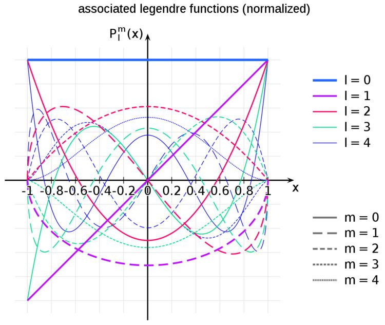
The first few associated Legendre functions

The first few associated Legendre functions, including those for negative values of m, are:

P 0 0 ( x ) = 1 P 1 − 1 ( x ) = − 1 2 P 1 1 ( x ) P 1 0 ( x ) = x P 1 1 ( x ) = − ( 1 − x 2 ) 1 / 2 P 2 − 2 ( x ) = 1 24 P 2 2 ( x ) P 2 − 1 ( x ) = − 1 6 P 2 1 ( x ) P 2 0 ( x ) = 1 2 ( 3 x 2 − 1 ) P 2 1 ( x ) = − 3 x ( 1 − x 2 ) 1 / 2 P 2 2 ( x ) = 3 ( 1 − x 2 ) P 3 − 3 ( x ) = − 1 720 P 3 3 ( x ) P 3 − 2 ( x ) = 1 120 P 3 2 ( x ) P 3 − 1 ( x ) = − 1 12 P 3 1 ( x ) P 3 0 ( x ) = 1 2 ( 5 x 3 − 3 x ) P 3 1 ( x ) = − 3 2 ( 5 x 2 − 1 ) ( 1 − x 2 ) 1 / 2 P 3 2 ( x ) = 15 x ( 1 − x 2 ) P 3 3 ( x ) = − 15 ( 1 − x 2 ) 3 / 2 P 4 − 4 ( x ) = 1 40320 P 4 4 ( x ) P 4 − 3 ( x ) = − 1 5040 P 4 3 ( x ) P 4 − 2 ( x ) = 1 360 P 4 2 ( x ) P 4 − 1 ( x ) = − 1 20 P 4 1 ( x ) P 4 0 ( x ) = 1 8 ( 35 x 4 − 30 x 2 + 3 ) P 4 1 ( x ) = − 5 2 ( 7 x 3 − 3 x ) ( 1 − x 2 ) 1 / 2 P 4 2 ( x ) = 15 2 ( 7 x 2 − 1 ) ( 1 − x 2 ) P 4 3 ( x ) = − 105 x ( 1 − x 2 ) 3 / 2 P 4 4 ( x ) = 105 ( 1 − x 2 ) 2

Recurrence formula

These functions have a number of recurrence properties:

( ℓ − m + 1 ) P ℓ + 1 m ( x ) = ( 2 ℓ + 1 ) x P ℓ m ( x ) − ( ℓ + m ) P ℓ − 1 m ( x ) 2 m x P ℓ m ( x ) = − 1 − x 2 [ P ℓ m + 1 ( x ) + ( ℓ + m ) ( ℓ − m + 1 ) P ℓ m − 1 ( x ) ] 1 1 − x 2 P ℓ m ( x ) = − 1 2 m [ P ℓ − 1 m + 1 ( x ) + ( ℓ + m − 1 ) ( ℓ + m ) P ℓ − 1 m − 1 ( x ) ] 1 1 − x 2 P ℓ m ( x ) = − 1 2 m [ P ℓ + 1 m + 1 ( x ) + ( ℓ − m + 1 ) ( ℓ − m + 2 ) P ℓ + 1 m − 1 ( x ) ] 1 − x 2 P ℓ m ( x ) = 1 2 ℓ + 1 [ ( ℓ − m + 1 ) ( ℓ − m + 2 ) P ℓ + 1 m − 1 ( x ) − ( ℓ + m − 1 ) ( ℓ + m ) P ℓ − 1 m − 1 ( x ) ] 1 − x 2 P ℓ m ( x ) = 1 2 ℓ + 1 [ − P ℓ + 1 m + 1 ( x ) + P ℓ − 1 m + 1 ( x ) ] 1 − x 2 P ℓ m + 1 ( x ) = ( ℓ − m ) x P ℓ m ( x ) − ( ℓ + m ) P ℓ − 1 m ( x ) 1 − x 2 P ℓ m + 1 ( x ) = ( ℓ − m + 1 ) P ℓ + 1 m ( x ) − ( ℓ + m + 1 ) x P ℓ m ( x ) 1 − x 2 d d x P ℓ m ( x ) = 1 2 [ ( ℓ + m ) ( ℓ − m + 1 ) P ℓ m − 1 ( x ) − P ℓ m + 1 ( x ) ] ( 1 − x 2 ) d d x P ℓ m ( x ) = 1 2 ℓ + 1 [ ( ℓ + 1 ) ( ℓ + m ) P ℓ − 1 m ( x ) − ℓ ( ℓ − m + 1 ) P ℓ + 1 m ( x ) ] ( x 2 − 1 ) d d x P ℓ m ( x ) = ℓ x P ℓ m ( x ) − ( ℓ + m ) P ℓ − 1 m ( x ) ( x 2 − 1 ) d d x P ℓ m ( x ) = − ( ℓ + 1 ) x P ℓ m ( x ) + ( ℓ − m + 1 ) P ℓ + 1 m ( x ) ( x 2 − 1 ) d d x P ℓ m ( x ) = 1 − x 2 P ℓ m + 1 ( x ) + m x P ℓ m ( x ) ( x 2 − 1 ) d d x P ℓ m ( x ) = − ( ℓ + m ) ( ℓ − m + 1 ) 1 − x 2 P ℓ m − 1 ( x ) − m x P ℓ m ( x )

Helpful identities (initial values for the first recursion):

P ℓ + 1 ℓ + 1 ( x ) = − ( 2 ℓ + 1 ) 1 − x 2 P ℓ ℓ ( x ) P ℓ ℓ ( x ) = ( − 1 ) ℓ ( 2 ℓ − 1 ) ! ! ( 1 − x 2 ) ( ℓ / 2 ) P ℓ + 1 ℓ ( x ) = x ( 2 ℓ + 1 ) P ℓ ℓ ( x )

with !! the double factorial.

Gaunt's formula

The integral over the product of three associated Legendre polynomials (with orders matching as shown below) is a necessary ingredient when developing products of Legendre polynomials into a series linear in the Legendre polynomials. For instance, this turns out to be necessary when doing atomic calculations of the Hartree–Fock variety where matrix elements of the Coulomb operator are needed. For this we have Gaunt's formula

This formula is to be used under the following assumptions:

1. the degrees are non-negative integers l , m , n ≥ 0
2. all three orders are non-negative integers u , v , w ≥ 0
3. u is the largest of the three orders
4. the orders sum up u = v + w
5. the degrees obey m ≥ n

Other quantities appearing in the formula are defined as

  2 s = l + m + n   p = max ( 0 , n − m − u )   q = min ( m + n − u , l − u , n − w )

The integral is zero unless

1. the sum of degrees is even so that s is an integer
2. the triangular condition is satisfied m + n ≥ l ≥ m − n

Dong and Lemus (2002) generalized the derivation of this formula to integrals over a product of an arbitrary number of Associated Legendre Polynomials.

Generalization via hypergeometric functions

These functions may actually be defined for general complex parameters and argument:

P λ μ ( z ) = 1 Γ ( 1 − μ ) [ 1 + z 1 − z ] μ / 2 2 F 1 ( − λ , λ + 1 ; 1 − μ ; 1 − z 2 )

where Γ is the gamma function and 2 F 1 is the hypergeometric function

2 F 1 ( α , β ; γ ; z ) = Γ ( γ ) Γ ( α ) Γ ( β ) ∑ n = 0 ∞ Γ ( n + α ) Γ ( n + β ) Γ ( n + γ )   n ! z n ,

They are called the Legendre functions when defined in this more general way. They satisfy the same differential equation as before:

( 1 − z 2 ) y ″ − 2 z y ′ + ( λ [ λ + 1 ] − μ 2 1 − z 2 ) y = 0.

Since this is a second order differential equation, it has a second solution, Q λ μ ( z ) , defined as:

Q λ μ ( z ) = π   Γ ( λ + μ + 1 ) 2 λ + 1 Γ ( λ + 3 / 2 ) 1 z λ + μ + 1 ( 1 − z 2 ) μ / 2 2 F 1 ( λ + μ + 1 2 , λ + μ + 2 2 ; λ + 3 2 ; 1 z 2 )

P λ μ ( z ) and Q λ μ ( z ) both obey the various recurrence formulas given previously.

Reparameterization in terms of angles

These functions are most useful when the argument is reparameterized in terms of angles, letting x = cos ⁡ θ :

P ℓ m ( cos ⁡ θ ) = ( − 1 ) m ( sin ⁡ θ ) m   d m d ( cos ⁡ θ ) m ( P ℓ ( cos ⁡ θ ) )

Using the relation ( 1 − x 2 ) 1 / 2 = sin ⁡ θ , the list given above yields the first few polynomials, parameterized this way, as:

P 0 0 ( cos ⁡ θ ) = 1 P 1 0 ( cos ⁡ θ ) = cos ⁡ θ P 1 1 ( cos ⁡ θ ) = − sin ⁡ θ P 2 0 ( cos ⁡ θ ) = 1 2 ( 3 cos 2 ⁡ θ − 1 ) P 2 1 ( cos ⁡ θ ) = − 3 cos ⁡ θ sin ⁡ θ P 2 2 ( cos ⁡ θ ) = 3 sin 2 ⁡ θ P 3 0 ( cos ⁡ θ ) = 1 2 ( 5 cos 3 ⁡ θ − 3 cos ⁡ θ ) P 3 1 ( cos ⁡ θ ) = − 3 2 ( 5 cos 2 ⁡ θ − 1 ) sin ⁡ θ P 3 2 ( cos ⁡ θ ) = 15 cos ⁡ θ sin 2 ⁡ θ P 3 3 ( cos ⁡ θ ) = − 15 sin 3 ⁡ θ P 4 0 ( cos ⁡ θ ) = 1 8 ( 35 cos 4 ⁡ θ − 30 cos 2 ⁡ θ + 3 ) P 4 1 ( cos ⁡ θ ) = − 5 2 ( 7 cos 3 ⁡ θ − 3 cos ⁡ θ ) sin ⁡ θ P 4 2 ( cos ⁡ θ ) = 15 2 ( 7 cos 2 ⁡ θ − 1 ) sin 2 ⁡ θ P 4 3 ( cos ⁡ θ ) = − 105 cos ⁡ θ sin 3 ⁡ θ P 4 4 ( cos ⁡ θ ) = 105 sin 4 ⁡ θ

The orthogonality relations given above become in this formulation: for fixed m, P ℓ m ( cos ⁡ θ ) are orthogonal, parameterized by θ over [ 0 , π ] , with weight sin ⁡ θ :

∫ 0 π P k m ( cos ⁡ θ ) P ℓ m ( cos ⁡ θ ) sin ⁡ θ d θ = 2 ( ℓ + m ) ! ( 2 ℓ + 1 ) ( ℓ − m ) !   δ k , ℓ

Also, for fixed ℓ:

∫ 0 π P ℓ m ( cos ⁡ θ ) P ℓ n ( cos ⁡ θ ) csc ⁡ θ d θ = { 0 if  m ≠ n ( ℓ + m ) ! m ( ℓ − m ) ! if  m = n ≠ 0 ∞ if  m = n = 0

In terms of θ, P ℓ m ( cos ⁡ θ ) are solutions of

d 2 y d θ 2 + cot ⁡ θ d y d θ + [ λ − m 2 sin 2 ⁡ θ ] y = 0

More precisely, given an integer m ≥ 0, the above equation has nonsingular solutions only when λ = ℓ ( ℓ + 1 ) for ℓ an integer ≥ m, and those solutions are proportional to P ℓ m ( cos ⁡ θ ) .

Applications in physics: spherical harmonics

In many occasions in physics, associated Legendre polynomials in terms of angles occur where spherical symmetry is involved. The colatitude angle in spherical coordinates is the angle θ used above. The longitude angle, ϕ , appears in a multiplying factor. Together, they make a set of functions called spherical harmonics. These functions express the symmetry of the two-sphere under the action of the Lie group SO(3).

What makes these functions useful is that they are central to the solution of the equation ∇ 2 ψ + λ ψ = 0 on the surface of a sphere. In spherical coordinates θ (colatitude) and φ (longitude), the Laplacian is

∇ 2 ψ = ∂ 2 ψ ∂ θ 2 + cot ⁡ θ ∂ ψ ∂ θ + csc 2 ⁡ θ ∂ 2 ψ ∂ ϕ 2 .

When the partial differential equation

∂ 2 ψ ∂ θ 2 + cot ⁡ θ ∂ ψ ∂ θ + csc 2 ⁡ θ ∂ 2 ψ ∂ ϕ 2 + λ ψ = 0

is solved by the method of separation of variables, one gets a φ-dependent part sin ⁡ ( m ϕ ) or cos ⁡ ( m ϕ ) for integer m≥0, and an equation for the θ-dependent part

d 2 y d θ 2 + cot ⁡ θ d y d θ + [ λ − m 2 sin 2 ⁡ θ ] y = 0

for which the solutions are P ℓ m ( cos ⁡ θ ) with ℓ ≥ m and λ = ℓ ( ℓ + 1 ) .

Therefore, the equation

∇ 2 ψ + λ ψ = 0

has nonsingular separated solutions only when λ = ℓ ( ℓ + 1 ) , and those solutions are proportional to

P ℓ m ( cos ⁡ θ )   cos ⁡ ( m ϕ )         0 ≤ m ≤ ℓ

and

P ℓ m ( cos ⁡ θ )   sin ⁡ ( m ϕ )         0 < m ≤ ℓ .

For each choice of ℓ, there are 2ℓ + 1 functions for the various values of m and choices of sine and cosine. They are all orthogonal in both ℓ and m when integrated over the surface of the sphere.

The solutions are usually written in terms of complex exponentials:

Y ℓ , m ( θ , ϕ ) = ( 2 ℓ + 1 ) ( ℓ − m ) ! 4 π ( ℓ + m ) !   P ℓ m ( cos ⁡ θ )   e i m ϕ − ℓ ≤ m ≤ ℓ .

The functions Y ℓ , m ( θ , ϕ ) are the spherical harmonics, and the quantity in the square root is a normalizing factor. Recalling the relation between the associated Legendre functions of positive and negative m, it is easily shown that the spherical harmonics satisfy the identity

Y ℓ , m ∗ ( θ , ϕ ) = ( − 1 ) m Y ℓ , − m ( θ , ϕ ) .

The spherical harmonic functions form a complete orthonormal set of functions in the sense of Fourier series. It should be noted that workers in the fields of geodesy, geomagnetism and spectral analysis use a different phase and normalization factor than given here (see spherical harmonics).

When a 3-dimensional spherically symmetric partial differential equation is solved by the method of separation of variables in spherical coordinates, the part that remains after removal of the radial part is typically of the form

∇ 2 ψ ( θ , ϕ ) + λ ψ ( θ , ϕ ) = 0 ,

and hence the solutions are spherical harmonics.

Generalizations

The Legendre polynomials are closely related to hypergeometric series. In the form of spherical harmonics, they express the symmetry of the two-sphere under the action of the Lie group SO(3). There are many other Lie groups besides SO(3), and an analogous generalization of the Legendre polynomials exist to express the symmetries of semi-simple Lie groups and Riemannian symmetric spaces. Crudely speaking, one may define a Laplacian on symmetric spaces; the eigenfunctions of the Laplacian can be thought of as generalizations of the spherical harmonics to other settings.