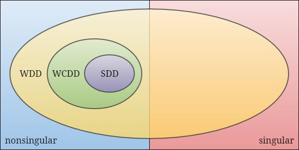
We say row i of a complex matrix A = ( a i j ) is strictly diagonally dominant (SDD) if | a i i | > ∑ j ≠ i | a i j | . We say A is SDD if all of its rows are SDD. Weakly diagonally dominant (WDD) is defined with ≥ instead.
The directed graph associated with an m × m complex matrix A = ( a i j ) is given by the vertices { 1 , … , m } and edges defined as follows: there exists an edge from i → j if and only if a i j ≠ 0 .
A complex square matrix A is said to be weakly chained diagonally dominant (WCDD) if
A is WDD andfor each row i of A , there exists a walk in the directed graph of A from i to an SDD row.Note that if i is itself an SDD row, the trivial walk i → i satisfies the second requirement in the above definition.
The matrix
( 1 − 1 1 − 1 1 ⋱ ⋱ − 1 1 ) is WCDD.
A WCDD matrix is nonsingular.
Proof: Let A = ( a i j ) be a WCDD matrix. Suppose there exists a nonzero x in the null space of A . Without loss of generality, let i 1 be such that | x i 1 | = 1 ≥ | x j | for all j . Since A is WCDD, we may pick a walk i 1 → i 2 → ⋯ → i m ending at an SDD row i m .
Taking modulii on both sides of
− a i 1 i 1 x i 1 = ∑ j ≠ i 1 a i 1 j x j and applying the triangle inequality yields
| a i 1 i 1 | ≤ ∑ j ≠ i 1 | a i 1 j | | x j | ≤ ∑ j ≠ i 1 | a i 1 j | , and hence row i 1 is not SDD. Moreover, since A is WDD, the above chain of inequalities holds with equality so that | x j | = 1 whenever a i 1 j ≠ 0 . Therefore, | x i 2 | = 1 . Repeating this argument with i 2 , i 3 , etc., we find that i m is not SDD, a contradiction. ◻
Recalling that an irreducible matrix is one whose associated directed graph is strongly connected, a trivial corollary of the above is that an irreducibly diagonally dominant matrix (i.e., an irreducible WDD matrix with at least one SDD row) is nonsingular.
The following are equivalent:
A is a WDD M-matrix. A is a nonsingular WDD L-matrix; A is a WCDD L-matrix;In fact, WCDD L-matrices were studied (by James H. Bramble and B. E. Hubbard) as early as 1964 in a journal article in which they appear under the alternate name of matrices of positive type.
Moreover, if A is an n × n WCDD L-matrix, we can bound its inverse as follows:
∥ A − 1 ∥ ∞ ≤ ∑ i [ a i i ∏ j = 1 i ( 1 − u j ) ] − 1 where
u i = 1 | a i i | ∑ j = i + 1 n | a i j | . Note that u n is always zero and that the right-hand side of the bound above is ∞ whenever one or more of the constants u i is one.
Tighter bounds for the inverse of a WCDD L-matrix are known.
Due to their relationship with M-matrices (see above), WCDD matrices appear often in practical applications. Some examples are given below.
Consider a Markov chain on the finite state space { 1 , … , m } . Let { π } be a (finite) set of stationary policies and P ( π ) be the transition matrix for the chain under policy π . Let ρ ( π ) ∈ [ 0 , 1 ] m denote an m -vector corresponding to the discount factor at each state of the Markov chain. Because each P ( π ) is a right stochastic matrix, { I − diag ( ρ ( π ) ) P ( π ) } is a family of WDD L-matrices. Convergence of R. A. Howard's policy iteration algorithm to the solution of a Markov decision process is guaranteed whenever this family consists only of inverse-positive matrices. As mentioned in a previous section, this occurs if and only if each member of the family is WCDD.
WCDD L-matrices arise naturally from monotone approximation schemes for partial differential equations.
For example, consider the one-dimensional Poisson problem
u ′ ′ ( x ) = f ( x ) for
x ∈ ( 0 , 1 ) with Dirichlet boundary conditions u ( 0 ) = u ( 1 ) = 0 . Letting { 0 , h , 2 h , … , 1 } be a numerical grid (for some positive h that divides unity), a monotone finite difference scheme for the Poisson problem takes the form of
− A u → = h 2 f → where
f → j = f ( j h ) and
A = ( 2 − 1 − 1 2 − 1 − 1 2 − 1 ⋱ ⋱ ⋱ − 1 2 − 1 − 1 2 ) . Note that A is a WCDD L-matrix.