Viola–Jones object detection framework

Problem description

The problem to be solved is detection of faces in an image. A human can do this easily, but a computer needs precise instructions and constraints. To make the task more manageable, Viola–Jones requires full view frontal upright faces. Thus in order to be detected, the entire face must point towards the camera and should not be tilted to either side. While it seems these constraints could diminish the algorithm's utility somewhat, because the detection step is most often followed by a recognition step, in practice these limits on pose are quite acceptable.

Feature types and evaluation

The characteristics of Viola–Jones algorithm which make it a good detection algorithm are:

Robust – very high detection rate (true-positive rate) & very low false-positive rate always.

Real time – For practical applications at least 2 frames per second must be processed.

Face detection only (not recognition) - The goal is to distinguish faces from non-faces (detection is the first step in the recognition process).

The algorithm has four stages:

1. Haar Feature Selection
2. Creating an Integral Image
3. Adaboost Training
4. Cascading Classifiers

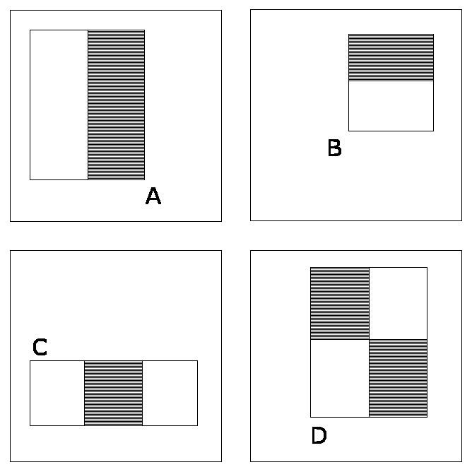
The features sought by the detection framework universally involve the sums of image pixels within rectangular areas. As such, they bear some resemblance to Haar basis functions, which have been used previously in the realm of image-based object detection. However, since the features used by Viola and Jones all rely on more than one rectangular area, they are generally more complex. The figure on the right illustrates the four different types of features used in the framework. The value of any given feature is the sum of the pixels within clear rectangles subtracted from the sum of the pixels within shaded rectangles. Rectangular features of this sort are primitive when compared to alternatives such as steerable filters. Although they are sensitive to vertical and horizontal features, their feedback is considerably coarser.

1. Haar Features – All human faces share some similar properties. These regularities may be matched using Haar Features.

A few properties common to human faces:

The eye region is darker than the upper-cheeks.

The nose bridge region is brighter than the eyes.

Composition of properties forming matchable facial features:

Location and size: eyes, mouth, bridge of nose

Value: oriented gradients of pixel intensities

The four features matched by this algorithm are then sought in the image of a face (shown at left).

Rectangle features:

Value = Σ (pixels in black area) - Σ (pixels in white area)

Three types: two-, three-, four-rectangles, Viola & Jones used two-rectangle features

For example: the difference in brightness between the white &black rectangles over a specific area

Each feature is related to a special location in the sub-window

2. An image representation called the integral image evaluates rectangular features in constant time, which gives them a considerable speed advantage over more sophisticated alternative features. Because each feature's rectangular area is always adjacent to at least one other rectangle, it follows that any two-rectangle feature can be computed in six array references, any three-rectangle feature in eight, and any four-rectangle feature in nine.

The integral image at location (x,y), is the sum of the pixels above and to the left of (x,y), inclusive.

Learning algorithm

The speed with which features may be evaluated does not adequately compensate for their number, however. For example, in a standard 24x24 pixel sub-window, there are a total of M = 162 , 336 possible features, and it would be prohibitively expensive to evaluate them all when testing an image. Thus, the object detection framework employs a variant of the learning algorithm AdaBoost to both select the best features and to train classifiers that use them. This algorithm constructs a “strong” classifier as a linear combination of weighted simple “weak” classifiers.

h ( x ) = sign ( ∑ j = 1 M α j h j ( x ) )

Each weak classifier is a threshold function based on the feature f j .

h j ( x ) = { − s j if  f j < θ j s j otherwise

The threshold value θ j and the polarity s j ∈ ± 1 are determined in the training, as well as the coefficients α j .

Here a simplified version of the learning algorithm is reported:

Input: Set of N positive and negative training images with their labels ( x i , y i ) . If image i is a face y i = 1 , if not y i = − 1 .

1. Initialization: assign a weight w 1 i = 1 N to each image i .
2. For each feature f j with j = 1 , . . . , M
   1. Renormalize the weights such that they sum to one.
   2. Apply the feature to each image in the training set, then find the optimal threshold and polarity θ j , s j that minimizes the weighted classification error. That is θ j , s j = arg ⁡ min θ , s ∑ i = 1 N w j i ε j i where ε j i = { 0 if  y i = h j ( x i , θ j , s j ) 1 otherwise
   3. Assign a weight α j to h j that is inversely proportional to the error rate. In this way best classifiers are considered more.
   4. The weights for the next iteration, i.e. w j + 1 i , are reduced for the images i that were correctly classified.
3. Set the final classifier to h ( x ) = sign ( ∑ j = 1 M α j h j ( x ) )

Cascade architecture

On average only 0.01% of all sub-windows are positive (faces)

Equal computation time is spent on all sub-windows

Must spend most time only on potentially positive sub-windows.

A simple 2-feature classifier can achieve almost 100% detection rate with 50% FP rate.

That classifier can act as a 1st layer of a series to filter out most negative windows

2nd layer with 10 features can tackle “harder” negative-windows which survived the 1st layer, and so on…

A cascade of gradually more complex classifiers achieves even better detection rates. The evaluation of the strong classifiers generated by the learning process can be done quickly, but it isn’t fast enough to run in real-time. For this reason, the strong classifiers are arranged in a cascade in order of complexity, where each successive classifier is trained only on those selected samples which pass through the preceding classifiers. If at any stage in the cascade a classifier rejects the sub-window under inspection, no further processing is performed and continue on searching the next sub-window. The cascade therefore has the form of a degenerate tree. In the case of faces, the first classifier in the cascade – called the attentional operator – uses only two features to achieve a false negative rate of approximately 0% and a false positive rate of 40%. The effect of this single classifier is to reduce by roughly half the number of times the entire cascade is evaluated.

In cascading, each stage consists of a strong classifier. So all the features are grouped into several stages where each stage has certain number of features.

The job of each stage is to determine whether a given sub-window is definitely not a face or may be a face. A given sub-window is immediately discarded as not a face if it fails in any of the stages.

A simple framework for cascade training is given below:

User selects values for f, the maximum acceptable false positive rate per layer and d, the minimum acceptable detection rate per layer.

User selects target overall false positive rate Ftarget.

P = set of positive examples

N = set of negative examples

F(0) = 1.0; D(0) = 1.0; i = 0 while F(i) > Ftarget i++ n(i) = 0; F(i)= F(i-1) while F(I) > f x F(i-1) n(i) ++ use P and N to train a classifier with n(I) features using AdaBoost Evaluate current cascaded classifier on validation set to determine F(i) & D(i) decrease threshold for the ith classifier until the current cascaded classifier has a detection rate of at least d x D(i-1) (this also affects F(i)) N = ∅ if F(i) > Ftarget then evaluate the current cascaded detector on the set of non-face images and put any false detections into the set N.

The cascade architecture has interesting implications for the performance of the individual classifiers. Because the activation of each classifier depends entirely on the behavior of its predecessor, the false positive rate for an entire cascade is:

F = ∏ i = 1 K f i .

Similarly, the detection rate is:

D = ∏ i = 1 K d i .

Thus, to match the false positive rates typically achieved by other detectors, each classifier can get away with having surprisingly poor performance. For example, for a 32-stage cascade to achieve a false positive rate of 10 − 6 , each classifier need only achieve a false positive rate of about 65%. At the same time, however, each classifier needs to be exceptionally capable if it is to achieve adequate detection rates. For example, to achieve a detection rate of about 90%, each classifier in the aforementioned cascade needs to achieve a detection rate of approximately 99.7%.

Advantages of Viola–Jones algorithm

Efficient feature selection

Scale and location invariant detector

Instead of scaling the image itself (e.g. pyramid-filters), we scale the features.

Such a generic detection scheme can be trained for detection of other types of objects (e.g. cars, hands)

Disadvantages of Viola–Jones algorithm

Detector is most effective only on frontal images of faces

It can hardly cope with 45° face rotation both around the vertical and horizontal axis.

Sensitive to lighting conditions

We might get multiple detections of the same face, due to overlapping sub-windows.

Related face detection and tracking algorithm

A method similar to Viola–Jones but that can better detect and track tilted and rotated faces is the KLT algorithm. Here numerous feature points are acquired by first scanning the face. These points then may be detected and tracked even when the face is tilted or turned away from the camera, something Viola–Jones has difficulty doing due to its dependence on rectangles.

Improvements over the Viola–Jones algorithm

An improved algorithm on Viola–Jones object detector

MATLAB implementation of Viola–Jones algorithm

OpenCV implementation of Viola–Jones algorithm

Haar Cascade Detection in OpenCV

Cascade Classifier Training in OpenCV

Citations of the Viola–Jones algorithm in Google Scholar

Implementing the Viola–Jones Face Detection Algorithm by Ole Helvig Jensen

Adaboost Explanation from ppt by Qing Chen, Discovery Labs, University of Ottawa and a video lecture by Ramsri Goutham.

Video link -